Espanhol (pdf)
 Artigo em XML
 Referências do artigo
 Enviar este artigo por email
 Citado por SciELO
  Citado por Google
  Similares em
SciELO
Similares em
SciELO  Similares em Google
 Permalink
Introduction
The real exchange rate (RER) and its misalignment from its long-term equilibrium are key inputs for assessing a country’s macroeconomic imbalance. The equilibrium real exchange rate (ERER) helps policymakers to deter- mine whether nominal exchange rate movements obey to temporary shocks that are likely to dissipate in the short term or are determined by more permanent changes in fundamental macroeconomic variables (Clark & MacDonald, 1998). In this sense, economic theory has approached the estimation of an RER long-term (or equilibrium) path through multiple methodologies. Given the multiple notions of equilibrium, a problem that arises is that the ERER estimates span over too many mixed results. Additionally, the results will still depend on several modeling assumptions, even when considering only a particular methodology (Adler & Grisse, 2017).
The literature has developed different methodologies to define and approach the ERER notion (Clark & MacDonald 1998; De Grauwe & Mongelli, 2005; Edwards, 1989; Isard, 2007; Obstfeld & Rogoff, 1996; Sarno & Taylor, 2003, among many others). The first, and one of the most commonly used, is the purchasing power parity (PPP), which is a generalization of the law of one price. A second one is the Fundamental Equilibrium Exchange Rate (FEER), which refers to the concept of medium-term equilibrium (Saxegaard et al., 2007; Rubaszek & Rawdanowicz, 2009). According to Fidora et al. (2021), it is obtained from the required adjustment of the exchange rate to equalize the medium-term sustainable value of the current account with its cyclically adjusted value. Stein (1990) proposed a third methodology named the natural real exchange rate (NATREX) approach, which defines the “natural” RER as “the RER that ensures the equilibrium of the balance of payments in the absence of cyclical factors, speculative capital movements and changes in international reserves”. The NATREX ensures internal and external equilibriums in the long run, specifically, when a country’s GDP converges to its potential level (or zero output gap), and the country’s current account attains a sustainable level. The fourth methodology is called Behavioral Equilibrium Exchange Rate (BEER), which uses cointegrated econometric methods to estimate an ERER that is determined by the long-term dynamics of the RER and its fundamentals.
This paper focuses on the BEER approach, as it is a methodology that uses economic fundamentals to explain the underlying structural movements of the ERER and derives a real exchange rate gap (or misalignment). This methodology is additionally utilized as an IMF’s tool for exchange rate assessments.1 According to Adler and Grisse (2017), a fundamental weakness of BEER models lies in the fact that structural macroeconomic models often incorporate multiple variables as potential explanatory variables for real exchange rates. Due to data limitations, it is often impossible (or impractical) to include all of these variables in the regression. The issue of model uncertainty arises due to the direct dependence of equilibrium rates and estimated coefficients on the particular model being estimated by the researcher. To ad- dress this, we establish five groups of multiple fundamentals that, according to the literature, best explain ERER movements: Indebtedness, Fiscal aggregates, Productivity, Terms-of-Trade (TOT) and Interest Rate Differentials. For each of the groups, we use several proxies.2 We estimated real exchange rate vector error correction (VEC) models3for all possible combinations of the fundamental variables across groups (always keeping one variable for each group of fundamentals). Thus, conducting iterations over the different variable specifications among each group results in 18,144 models (for further details, see Section III). It must be noted we are addressing only one specific and narrow type of model uncertainty, specifically the combinations of con- temporaneous variables of each type. From these models, we filter out those that exhibit coefficients with the expected sign and significance, as well as those whose residuals satisfy the non-autocorrelation, homoscedasticity, normality, and stationarity assumptions. We construct an empirical distribution for the RER equilibrium and its misalignment from the selected models.
It is important to note that the results can vary at some points in time due to fluctuations, sometimes significant, in the ERER of alternative specifications. Furthermore, because the long-term level of the RER (equilibrium) is an unobserved variable, selecting the most appropriate model is challenging since there is no reference that permits to evaluate the magnitude of the estimate’s error. Therefore, this paper explores the robustness of Colombia’s equilibrium real exchange rate using the BEER approach.
The document is organized as follows. The following section discusses the related literature and our contributions. The third section describes the study data and explains all the proxies used as fundamentals. The fourth section presents and derives the empirical strategy. The results are presented and discussed in the fifth section, and the conclusion and main findings are covered in the last section.
Literature Review
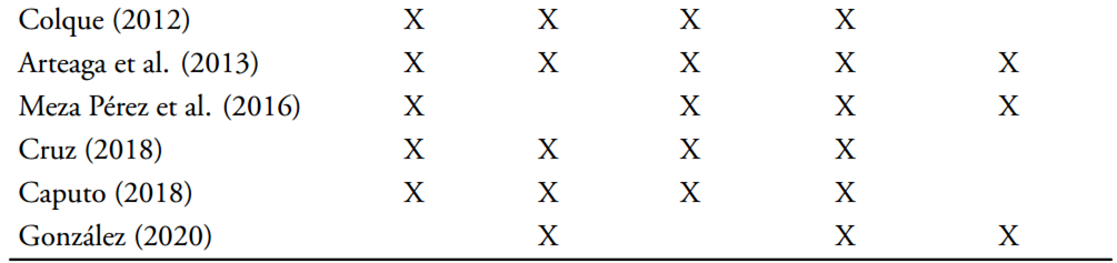
This section presents a literature review of papers that are closely related to the subject matter of this research. These papers have been selected because they offer estimates of ERER through a cointegration approach. A more detailed overview of variables that represents a relevant channel in the real exchange rate literature is provided in Table A1 of the appendix. The approach carried out in this document is framed within the BEER, as defined by Clark and MacDonald (1998). Under this methodology, the ERER is constructed based on reduced-form models and time series estimates that seek to capture how different variables determine the dynamics of the RER. In this sense, these models not only seek to explain the medium- and long-term dynamics of the exchange rate but also its short-term dynamics. According to this notion of equilibrium, the ERER varies over time and is specified as a function of its fundamentals, determined by macroeconomic theory. Using a VEC model, the authors distinguish between permanent (terms of trade, relative prices on non-traded to traded goods, the stock of net foreign assets, and a proxy for the risk premium) and transitory (interest rate differential) com- ponents of RER fundamentals for the G-3 currencies. They found that the BEER model was consistent with the theory as it explained actual movements of the real effective exchange rate.
Maeso-Fernández et al. (2002) present an empirical analysis of the medium- term determinants of the euro exchange rate. The empirical analysis derives a BEER and a Permanent Equilibrium Exchange Rate (PEER).4 Both models were rather similar, with the PEERs being smoother than the BEERs. Their study findings show that the variables of productivity, differentials in real interest rates, relative fiscal stance, and the real oil price have a significant influence on the euro’s effective exchange rate. Ricci and MacDonald (2003) estimate a VEC model to find the ERER in South Africa using quarterly data for the period 1970Q1 to 2002Q1. These authors consider the real interest rate differential, relative GDP per capita, real commodity prices, an openness indica- tor, the fiscal balance, and the net foreign assets (NFA) as determinants of the real exchange rate. Clark and MacDonald (2004) extend the BEER approach by using real interest rate differential, net foreign assets, and the relative price of non-traded/traded goods as economic fundamentals. Johansen cointegration methods are employed to decompose the fundamentals into transitory and permanent components. The permanent component was used to estimate the PEER for the pound sterling, U.S. dollar and Canadian dollar. For the U.S. dollar and the Canadian dollars, they found that the BEER and the PEER are remarkably similar and generally follow the observed exchange rate.
Paiva (2006) estimates the BEER model for Brazil through a VEC specification for the period 1970 to 2004. The author considers the relative price of non-tradable to tradable, terms of trade, real interest rate differentials, the net foreign assets position, and the relative stock of public domestic debt as the fundamentals related to the real exchange rate. After estimating the unit root test, the author determined that the real interest rate differential is stationary. These findings indicate that the absolute value of the interest rate differential coefficient in the cointegrating equation is relatively small, suggesting a minimal contribution.
Lee et al. (2008) describes all the methods used by the International Monetary Fund to evaluate the misalignment of the exchange rate in member countries. These authors classify the use of cointegration methods between the RER and its fundamentals within the Equilibrium Real Exchange Rate methodology and describe an estimate of a panel VEC for 48 countries with annual data for the period 1980-2004. Caputo and Núñez (2008) estimate an equation for Chile’s RER based on its fundamental determinants using quarterly data for the period 1977-2007. These authors use the ratio between tradable and non-tradable productivity, Government spending, ToT, NFA, and tariff levels as fundamentals.
Bénassy-Quéré et al. (2009a) study the robustness of the equilibrium exchange rate estimations from BEER methods. They investigate industrial an emerging countries’ potential fundamentals that include net foreign asset position, relative productivity, interest-rate differential, and terms of trade. From this analysis, they conclude that BEER estimations are robust to several tests and that the productivity proxy tends to be the more sensible option.
Bussiére et al. (2010) carry out an analysis of the main methodologies for estimating the RER equilibrium, with a focus on describing the most recent methodological advances that allow an improvement in the estimation. For the estimation of a reduced form of the RER and its determinants, these authors recommend taking into account fundamentals related to trade restrictions, productivity, government consumption, capital formation, NFA, and commodity prices. For each combination of fundamentals, they select only those models that satisfy the criteria for the existence of a long-run relation- ship, those with significant level elasticities, and those whose coefficient meets the expected sign in line with the theoretical restrictions.
Adler and Grisse (2017) explore the robustness of BEER models addressing the issue of model uncertainty, which aligns with our research. They inves tigate this robustness by including country fixed effects and evaluate the sensitivity of the estimated coefficients to different combinations of economic fundamentals underlying the RER. In their estimation, the authors consider several variables such as trade balance, terms of trade, real interest rate, productivity, private credit, population growth, output gap, trade openness, old age dependency rate, net foreign assets, government consumption, GDP per capita, fiscal balance, fertility rate, and central bank reserves. They estimate thousands of RER regressions over all possible combinations of the aforementioned fundamentals, ranging from models with one or two variables to the inclusion of all variables. Finally, they construct the distribution of the misalignment across all cointegrating models to identify the median of the estimation. Their main finding is that the estimated coefficients and, consequently, the implied equilibrium exchange rates, are sensitive to several modeling assumptions. Therefore, it is important to exercise caution when interpreting the point estimates of equilibrium exchange rates and to explore how the effects of specific variables depend on the model’s specification. The reasons addressed by Adler and Grisse (2017) were the main motivation for our methodological approach.
Several papers have attempted to estimate ERER and RER misalignments for Colombia. Oliveros and Huertas-Campos (2003) were among the first to perform a VEC estimation to find the equilibrium RER with annual data during the period 1958-2001. The determinants used as a proxy for the Balassa- Samuelson effect were NFA, interest rate differential, and the relationship be- tween tradable and non-tradable prices. Echavarría et al. (2005) estimated a VEC with annual data for the period 1962-2004 and considered the following long-term determinants (fundamentals) of the RER: NFA, GDP growth differential between Colombia and the US, ToT, Government consumption, US RER and Colombia’s nominal COP/USD exchange rate. Later, Echavarría et al. (2007) estimated a common trend approach associated with a Structural VEC model to obtain an ERER for Colombia. In this case, they used annual data for the period 1962-2005 and the following fundamentals for the RER: NFA, ToT, and an openness indicator.
Alonso et al. (2008) proposed easy-to-follow alternative measures to periodically assess the evolution of the RER. A preliminary analysis was conducted to determine the degree to which its various methodologies were misaligned with respect to their long-term level. Puyana-Martínez (2010) estimated the relationship between relative tradable and non-tradable productivities using data from the Colombian manufacturing sector. The author identifies a strong correlation between this indicator and the RER for the period 1992-2004. Arteaga et al. (2013) studied the behavior of the RER between 1994 and 2012 using a cointegration model. Their results highlight the importance of national terms of trade and the Balassa-Samuelson effect in explaining the real appreciation observed since the end of 2003. Our work adds to this strand of literature by studying the dynamics of the real exchange rate in Colombia over a more recent period (2000-2019) and its robustness when changing variable specifications.
Data
We use quarterly data from the first quarter of 2000 to the fourth quarter of 2019. The selection of the period is constrained by the availability of information and the fact that Colombia has adopted a flexible exchange rate within the frame of an inflation-targeting regime. The variables in the dataset were seasonally adjusted using the Census X-13 method (if seasonality is present). All variables that were not percentages were introduced in their logarithmic transformation so that their magnitudes were comparable.
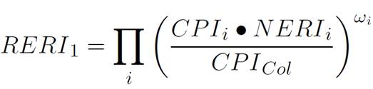
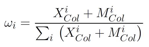
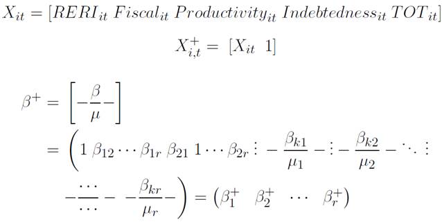
As previously stated, we classify all our variable specifications into five different groups (Table 1) and subsequently estimate the VEC models by iterating over the variables within each group. Each group represents a theoretically intuitive and relevant channel in the literature (Table A1 of the appendix). Given that each type corresponds to one of the relevant channels in the RER literature, we consider it appropriate to include one variable from each group in our candidate specifications. The variable in the first group is the logarithm of the real exchange rate index (RERI) that uses total weights5and the CPI as the deflator for all countries (section A of the appendix provides details on its construction). It is assumed to be the most endogenous because it responds to all the fundamentals. All the variables used, their detailed description and their source can be found in Table A3 of the appendix.
Fundamental determinants of ERER
This section will provide a comprehensive description of the groups of fundamental drivers, along with their constituent variables., The classification of the five fundamental variables that are widely recognized in the literature as the main drivers of the RER is presented in Table A1 of the appendix.
Fiscal. The relationship between the real exchange rate and fiscal policy has been analyzed from multiple perspectives in the literature. In the first place, Keynesian theories framed in the Mundell-Fleming model imply that a positive fiscal shock increases domestic demand. Along with sticky wages and prices, this induces a real appreciation (Mundell, 1963; Fleming, 1962; Badia & Segura- Ubiergo, 2014). In the case of real business cycle models, government spending shocks crowd out domestic private consumption, increasing labor supply and appreciating the real exchange rate (Backus et al., 1995). However, other studies, such as Ravn et al. (2007) and Kollmann (2010), find opposite results. Maeso- Fernández et al. (2006) and Badia and Segura-Ubiergo (2014) also highlight the role of the composition of government spending. In particular, the latter authors note that increases in government spending on non-tradable goods, financed either by taxes or debt, will generate a real appreciation. On the other hand, the effect of raises in public investment is unclear. As Balassa (1964) and Samuelson (1964) pointed out, an increase in public investment may appreciate the RER if there are gains in productivity in the tradable sector, but it may depreciate the RER if there are disproportionate increases in productivity in the non-tradable sector. Moreover, if both tradable and non-tradable sectors experience similar gains in productivity, the RER will not be affected (Galstyan & Lane, 2009).
In this work, we follow the New-Keynesian approach, according to which an increase in public spending generates an appreciation of the real exchange rate (negative sign), as it is more frequently channeled towards non-tradable goods and services (De Gregorio & Wolf, 1994; De Gregorio et al., 1994; Froot & Rogoff, 1995). The channel can be described as follows: as the GDP and aggregate demand increase, there is a subsequent rise in the demand for labor and capital, leading to higher wages and marginal costs and, consequently, inflation, which implies an increase in the policy rate and capital inflows, and an appreciation of the exchange rate.
Productivity. The inclusion of a productivity variable is commonly motivated by the Balassa- Samuelson theory, according to which the bigger the productivity gap in traded goods production between two countries, the larger the wage and price of services differences and, “correspondingly, the greater the gap between purchasing-power parity and the equilibrium exchange rate.” (Balassa, 1964, p 586). Because total factor productivity is difficult to measure, De Broeck and Slok (2006) and Fischer (2004) employ labor productivity me sures in different sectors and find evidence that a rise in productivity implies a real appreciation of the respective currency. As most of our variables are defined as ratios with Colombia in the denominator, the expected sign for the coefficients in this set of variables is positive.
Table 1 Fundamental Group Variables
| Public consumption % GDP | quarters) Trade partners/COL index ratio | NFPS Spending % GDP | Per capita trade partners/COL index ratio Per capita relative index USA/Col GDP PPP Per capita ratio USA/Col |
| Indebtedness | Terms of Trade | Int. Rate Diff |
| Public external debt outstanding | Terms of Trade CE | Dif Assets-Prime |
| Total external debt | Terms of Trade PPI | Diff FTD 90 days |
| NFA prime Real GDP | Mining Terms of Trade | Diff FTD 360-Prime |
| NFA GDP | Implicit Real Oil Price | Diff FTD-Prime |
| Real NFA | Real Brent price | Diff FTD-3mlibor |
| NFA prime GDP Private external debt NFA prime Real CNG Outstanding Debt | National accounts | Terms of Trade |
Note: RERI: Real Exchange Rate Index; CNG: Central National Government; NFPS: Non-Financial Public Sector; T: Tradable; NT: Non- Tradable; PPP: Purchasing Power Parity; NFA: Net Foreign Assets; Prime: Prime rate; CE: Foreign Trade; PPI: Producer Price Index; FTD: Fixed-term Deposits; FTD360: Fixed-term Deposits 360 days’ rate; FTD3mlibor: Fixed-term Deposits 3-month LIBOR rate; GDP: Gross Domestic Product. See Table A3 of the appendix for a detailed description on each variable.
Source: Own elaboration.
Indebtedness. In this group, we include nine variables that offer different measures of indebtedness of the Colombian economy. This includes out- standing debt variables and Net Foreign Assets (NFA). In the case of the debt variables, the expected sign would be positive, as a more indebted country is perceived as riskier (Cosset & Roy, 1991). As emphasized by Ajevskis et al. (2014), “If a country is in a debtor’s position, net interest payments weigh on the current account balances. The latter requires strengthening international price competitiveness and a more depreciated real exchange rate.” (p. 104). Similarly, as Phillips et al. (2013) and Mano (2019) point out, NFA are expected to have a negative coefficient as a country with higher foreign borrowing (worse NFA position) requires a more depreciated RER to reduce its trade balance deficit.
Terms of Trade. Terms of trade proxy indicators should have negative signs. Neary (1988) indicates that more favorable terms of trade are associated with higher wealth and, thus, a more appreciated RER. According to Ajevskis et al. (2014), higher commodity terms of trade should lead to real exchange rate appreciation via real income effect. Calderón (2004) elaborates on this idea by stating that terms of trade improvements would increase tradable goods’ consumption and generate positive wealth effects that would reduce the sup- ply of labor in the non-tradable sector. This leads to a relative non-tradable goods price increase, thereby appreciating the RER.
Interest Rate Differentials. According to Adler and Grisse (2017) and Paiva (2006), real interest rate differentials should have a negative sign, which indicates that an increase in the differential will cause an appreciation of the RER. This is because a higher domestic interest rate relative to foreign interest rates offers investors higher returns in the country, thereby attracting foreign capital and, thus, an appreciated RER.
Empirical Strategy
We estimate thousands of Vector Error Correction (VEC) specifications for 2000Q1-2019Q4. Each model corresponds to a realization of all possible contemporaneous combinations of the fundamental variables across the groups described in part A of Section II (fixing one variable for each group
of fundamentals) for the RER specification. The latter is built as the multi- lateral RER index weighted by total non-traditional goods trade, deflated by the consumer price index (see section A of the appendix for further details). The estimated VEC corresponds to DRIFT models according to the usual notation (Arteaga et al., 2013; Johansen, 1992; Maeso-Fernández et al., 2006) with one lag and one cointegration relationship. 6
For this work, a maximum of lags p = 2 was established in the VAR (p = 1 in the VEC) to avoid losing an excessive number of degrees of freedom due to data limitations. In addition, we conduct unit root tests on all variables, and as shown in Table A2 of the appendix, all endogenous variables are non- stationary with integration order 1 (I (1)). Following Paiva (2006) and Arteaga et al. (2013), interest rate differentials variables are treated as exogenous as they are stationary (I (0)), and they are excluded from the cointegration vector. See Table A2 for the entire Unit Root Tests of all the variables in our VEC models.
Cointegration Tests
Once the VEC lags are defined, the cointegration test is applied using the trace test and the maximum eigenvalue test (eigen test) of Johansen (1992) for each resulting combination of one variable of each leading group, one variable for the exogenous Interest Rate Differentials group, and one constant. If at least one of the two tests concludes there is one cointegration relationship, the model is selected.
After the number of cointegration relationships for each combination of variables is established, we estimate all the VEC models with one cointegration relationship.
Model and Cointegration Vector Estimation
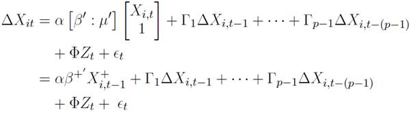
For the estimation of a VEC model, the following specification was used:
 (1)
(1)
where
i is the subscript of the model, p is the order in which the variables are lagged in the VAR representation, α is a matrix of dimension K × r containing the convergence speeds to equilibrium, and [β; µ] is the matrix of dimension (K + 1) × r that represents the concatenation between the matrix β(K × r), which contains the long-term relationships and the array µ(1× r) that contains the constant term. Γ l (l = 1, . . . , p - 1) are matrices K× K containing the short-term fit coefficients, Z is the vector of exogenous variables that, in this case, are associated with the group of rate differentials, and ϵ is the K×1 vector of errors.7
Real Equilibrium Exchange Rate and its Misalignment
The predicted value from the VEC model regression is interpreted as the ERER in the BEER literature. The ERER associated with each model is obtained from the models estimated in the previous section. The total equilibria are equivalent to the total number of possible models estimated. For the ERER calculation the linear combination in equation (2) between the vector (β +) and the observed data of each variable that composes it (X +) is performed. This estimate is done for each model i for each t
 (2)
(2)
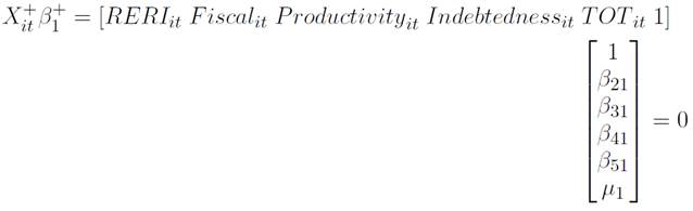
where β k,1 together with µ 1 are the coefficients of the first cointegration vector: β + associated with the model i. The equilibrium is noted by RERI ∗ to avoid confusion with the observed RERI.
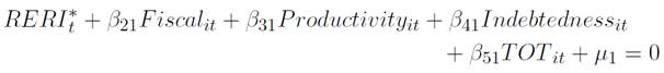
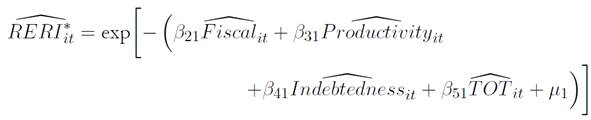
Considering that RERI has been transformed into logarithms and that the cointegration vector is normalized, the logarithm of the equilibrium of the i-th model is obtained in each t:
 (3)
(3)
Once the equilibrium has been calculated, the misalignment of model i is calculated for each time t as the percentage change between the observed exchange rate and the equilibrium rate.
Following the literature (Clark & MacDonald, 1998), a smoothed equilibrium measure is calculated. We use equation (3) but replace the right-hand side variables with the smoothed versions using the Hodrick and Prescott filter, denoted as x it . The aforementioned procedure is made to obtain the equilibrium that does not incorporate short-term movement of its fundamentals.
Then the smoothed misalignment is calculated as the percentage deviation between the observed exchange rate and the smoothed equilibrium rate.
Model Selection
After identifying all the misalignments, we filter out those models where 𝛽 1 + together with the exogenous component Φ do not meet the expected signs (as explained in Section II). The significance of the coefficients of the remaining models is evaluated, and the cases in which at least 4 out of 6 coefficients were significant (at 10% level) are selected. In addition to the sign and significance filter, all models that do not meet the criteria for non- autocorrelation, homoscedasticity, normality, and stationarity in the residuals are excluded.
Equilibrium and Misalignment Distribution
To obtain a central path of equilibrium and misalignment in each period of time, the selected models are grouped and their median is calculated for each t. This process is done for both smoothed and unsmoothed estimates. The equilibria are calculated for each time t, (t = 1, . . . , T ) and each model i, (i = 1, . . . , N ). The 20th and 80th percentiles are obtained in the same way and will represent the intervals around the central path (median). A matrix representation of this process is presented in Tables 2 and 3:
Results
This section begins by showing the distribution of coefficients across all models8 to test the robustness of the sign and the magnitude of the estimated coefficients to alternative model specifications. The different hypotheses on the signs of the coefficients associated with the variables discussed in Section II are empirically addressed. Then, from the selection of models that meet the criteria on sign, significance and residual assumptions (as discussed in Section III), the empirical distribution of equilibria and misalignments are shown across all the range of models. It is important to note that we are addressing only one specific and narrow type of model uncertainty: combinations of contemporaneous variables of each type.
Distribution of Coefficients
In section B of the appendix (Figures A1 through A4), we report the distribution of the estimated coefficients associated with variables within the cointegration vector and across models. The proportion of red to white shows the share of estimations with statistically significant coefficients at the 10% level. These distributions illustrate the robustness of the sign and magnitude of the estimated coefficients to alternative model specifications. A negative (positive) coefficient implies that increases in the corresponding variable are associated with a real effective appreciation (depreciation) of the RER.
Our results suggest that the terms of trade group variables are robustly linked to real exchange rates in the sense that their coefficients among all six variables are, on average, significant in 79% of all possible models. Furthermore, in approximately 76% of the total models they have the theoretically predicted sign (Figure A1). The latter result strongly supports the theory that higher commodity terms of trade should lead to real exchange rate appreciation via real income effect (Neary, 1988; Ajevskis et al., 2014).
In the productivity group (Figure A2), the variables with the highest percentage of significant coefficients across all possible model combinations (and with the expected sign) are the ones relating productivity measures between Colombia and its main trading partners. Indeed, among the two variables measuring the relative productivity of Colombia and that of its main trading partners, 98% and 95% of the models were significant and met the expected sign, respectively. The worst-performing productivity proxy in this group is the per-capita relative index between the US and Colombia, of which 45.8% is significant and, among those, 53.5% have the expected positive sign. It is worth noting that as our variables are defined as ratios with Colombia in the denominator, the expected sign for the coefficients in this set of variables is positive. As mentioned in Section II, the inclusion of a productivity variable is commonly motivated by the Balassa- Samuelson theory. Our results largely support both the theoretical and empirical evidence that a rise in productivity implies a real appreciation of the local currency.
With respect to the Indebtedness group of variables, they consistently exhibit the expected sign in most variables, specifically the ones including outstanding debt (Figure A3). Public external debt outstanding as percentage of the moving sum four quarters of nominal GDP in USD, and NFA as percentage of nominal GDP, are statistically significant in over 95% of the regressions and, approximately, 92% exhibit the expected sign (positive for the public debt outstanding and negative for the NFA/GDP). Total external debt is another outperformer, with 77% of the coefficients being significant and 75% of the total estimated models exhibiting the expected positive sign. It is worth noting that NFA times the prime interest rate divided by the sum of four quarters of the GDP (NFA prime GDP), NFA times the prime real interest rate deflated by US CPI (NFA prime real) and NFA times the prime interest rate as percentage of real GDP (NFA prime REAL GDP) exhibit a distribution with 54%, 47% and 38% of the models, respectively, having the expected sign.
Lastly, in the fiscal group, all variables considered are significant in more than 52% of the cases (Figure A4). In particular, the three variables related to Public Consumption (Public Consumption, Public Consumption as a percentage of GDP, and Public Consumption as a share of Total Consumption) predominantly exhibit the expected negative sign. These results support the works of Maeso-Fernández et al. (2006) and Badia and Segura-Ubiergo (2014), which highlight the role of the composition of government spending as “increases in government spending-whether tax or debt-financed-will result in a real appreciation if skewed toward non-tradable goods.” Our results also seem to support the New-Keynesian approach, which posits that an increase in public spending generates an appreciation of the real exchange rate (negative sign), as it is primarily channeled towards non-tradable goods and services (De Gregorio & Wolf, 1994; De Gregorio et al., 1994; Froot & Rogoff, 1995). In the long term, high government/public sector spending, mainly if it is financed by debt, may widen the interest rate differential between the economy and the rest of the world as it increases the country’s risk premium (Bouakez & Eyquem, 2015; Kollmann, 2002; Schmitt-Grohé & Uribe, 2003; Senhadji, 2003). This may lead to distortions in the economy and undermine market confidence in a currency. Colombia’s persistent fiscal deficit could explain the positive coefficients on CNG Spending, NFPS Spending, and NFPS Spending as a percentage of GDP.
Distribution of ERER and Misalignment
As discussed in Section 5.1, both the magnitude and sign of the estimated coefficients are sensitive to the combinations of variables in a particular regression. Thus, the model implied that the ERER will also depend on the chosen specification and each model would imply a different path for the equilibrium exchange rate. For that reason, we present the empirical distributions of ERER and smoothed ERER (Ricci & MacDonald, 2003). In a VEC model, the equilibrium relationship results from multiplying the cointegration vector found by the values of the variables at each moment in time. In the smoothed ERER, we use the cointegration vector of the VEC and multiply it by the smoothed variables9 to omit transient movements in them that should not lead to changes in the ERER.
Figure 1 shows the empirical distribution of ERER (Panel A) and the empiri cal distribution of smoothed ERER (Panel B). The median of these empirical distributions shows that the country experienced a reduction in ERER from 2004 to 2013. In addition, the complete distribution also exhibits a trend towards appreciation of the ERER during these years. This result is associated with higher terms of trade,10 some improvements in relative productivity, an increase of government spending11 and a reduction of external indebtedness as a percentage of GDP.12 Arteaga et al. (2013) found a similar trend for ERER by estimating a VEC model for Colombia between 1994Q2 and 2012. Our estimation also reveals that from 2014 to 2019, ERER increased amidst a negative shock to the terms of trade, higher external debt and a deterioration of net foreign assets.13
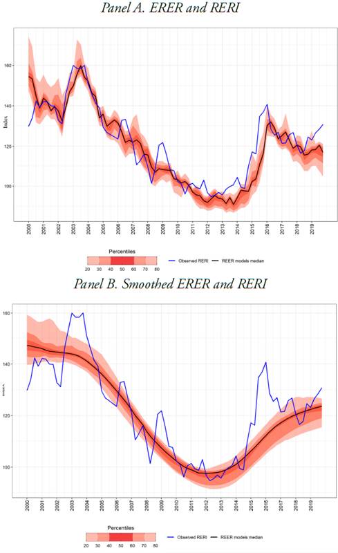
Note: Figures in both Panel A and Panel B cover the period 2000Q1-2019Q4. Panel B reports the ERER distribution that results from replacing the fundamentals by its long-term equilibriums (Hodrick-Prescott trend component). The widest bands correspond to the area between percentiles 20 and 80 of the distribution. Source: own elaboration.
Figure 1 Distribution of ERER and smoothed ERER
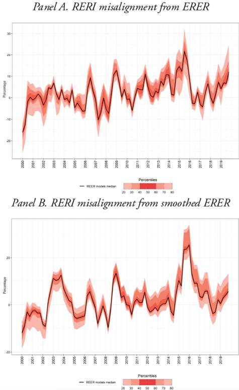
Figure 2 also presents the corresponding misalignment of RER. According to both methodologies, during the global financial crisis (2008-2009) and the oil price shock (2014-2015), there was a significant deviation of the RER from the equilibrium during the sample period. Additionally, taking into account the flexible exchange rate regime adopted in Colombia since 2000, the RER oscillated around the equilibrium during our sample period.
Conclusions
The approach carried out in this work is framed within the Behavioral Equilibrium Exchange Rate (BEER), as defined by Clark and MacDonald (1998). Under this methodology, the equilibrium real exchange rate (ERER) is constructed based on reduced-form models and time series estimates that seek to capture how different variables determine the RER’s dynamics. According to this notion of equilibrium, the ERER varies over time and is specified as a function of its fundamentals, determined by macroeconomic theory. The literature (i.e., Adler & Grisse, 2017; Phillips et al., 2013) has identified that the estimation of the ERER through the BEER methodology tends to be extremely sensitive to the model specification and the set of fundamentals used. In general, BEER models suggest several variables as potential drivers of real exchange rates. This gives rise to the issue of model uncertainty, as coefficients and equilibrium rates depend on the particular specification being estimated. To address this issue, we establish five groups of multiple fundamentals that, according to the literature, best explain ERER movements: Indebtedness, Fiscal aggregates, Productivity, Terms-of-Trade, and Interest Rate Differentials. We use several proxies for each group and estimate real exchange rate VEC models for all possible combinations of the fundamental variables across groups (fixing one variable for each group of fundamentals). From a set of filtered models, we derive an empirical distribution of ERER that allows us to determine with greater certainty, among hundreds of plausible economic specifications, whether the real exchange rate is in equilibrium or misaligned. It is important to note that we address only one specific and narrow type of model uncertainty: combinations of contemporaneous variables of each type. To address other uncertainty sources, future works
should also consider robustness among different methodological specifications, such as Autoregressive Distributed Lag Model (ARDL), Fully Modified OLS (FMOLS), or Dynamic OLS (DOLS), among others.
The median of the empirical distributions shows that from 2004 to 2013, Colombia experienced a reduction in ERER and a trend towards its appreciation. This result is associated with higher terms of trade, a slight improvement in relative productivity, an increase in government spending and a reduction in external indebtedness as a share of GDP. Our estimations also reveal that between 2014 and 2019, ERER depreciated as a consequence of a negative terms-of-trade shock, higher external debt and the deterioration of net foreign assets.