


 Inglês (pdf)
 Artigo em XML
 Referências do artigo
 Enviar este artigo por email
 Citado por SciELO
  Citado por Google
  Similares em
SciELO
Similares em
SciELO  Similares em Google
 Permalink
Introduction
Chemists study reaction mechanisms (also called reaction networks [1, 2]), using mathematical tools to solve, quantitatively or qualitatively, the differential equations associated with those networks. The existence of quantitative (analytical) solutions to these differential equations is desirable but limited to a small set of chemical networks [3]. Qualitative analysis, for example, linear stability analysis [4], Stoichiometric Network Analysis (SNA) [1, 2], or more recently, Frank inequality for homochiral networks [5, 6], gives us valuable information, but when the mechanisms involve many species and reactions, these qualitative analyses are hard to carry out. One more practical approach, although not a general solution, is to simulate the chemical network of interest under particular conditions. This means to solve, numerically, the differential equations associated with the network [7]. This is a kind of exhaustive search [8] that produces a particular solution and usually requires a significant quantity of numerical work, the kind of work that it is quickly done, most of the time, by computers. The good thing about exhaustive search is that, in most of the cases, it finds solutions. This is an option when no other mathematical tools can be used to know the behavior of a model. Notice that simulations are also one way to test the results and predictions found with the qualitative tools of mathematics.
The computer simulation of any chemical mechanism requires to translate the process into a machine-readable format. The chemists need to learn how to transform their knowledge into a piece of code that a programming language could understand. Coding is a skill that takes time to be mastered. Thus, a user-friendly computer program is a nice alternative.
Software specialized in the simulation of reaction networks already exist. Five aleatory examples are COPASI [9], a free program available from http://copasi.org/, which has excellent capabilities, including SNA; Chemsimul [10], a licensed program available at http://chemsimul.dk/; KPP [11], a free program available at http://people.cs.vt.edu/asandu/Software/Kpp/; KinSim, a simulation tool that is specifically oriented to environmental studies, and which is pretended to be used as a pedagogical tool in higher education [12]; and ReactLab KINETICS, a licensed and expensive software [13]. Although these, and many others, are mature and excellent pieces of software, sometimes they become cumbersome to work with, or excessively complex, or they lack suitable documentation, or they are simply more than we need. In our particular work, we need to experiment with many different parameters for a reaction network; thus, we require a way to modify them often. Chemkinlator was designed thinking in this kind of work. That is why we tried to make it very simple to use.
We do not pretend to review the available software for chemical kinetics simulations. We want to contribute with a new piece of software, which could be of use for people interested in chemical kinetics, especially those interested in teaching chemical kinetics at the university level. This software is open source, which means that the user has access to the code. If the user has different needs to those that the software accomplishes, the user may modify it accordingly.
Chemkinlator interface consists of a single window where all parameters of the reaction network are at one click of distance to be selected and modified. Chemkinlator, in its main window (Tab), assumes that any reaction network can be written as a list of reactions occurring in a closed reactor with no explicit effect of temperature. Nevertheless, more complex simulations can be executed by more complex Tabs, which are layered on top of the interface. Currently, Chemkinlator has included two additional Tab s: Bifurcation, where bifurcation diagrams [14, 15, 16] as a function of the rate constants can be computed and displayed; and Flow/Temperature, where the effects of flow and temperature, in a Continuous-flow well-Stirred Tank Reactor (CSTR) [17], can be simulated.
Chemkinlator comes with several examples of reactions, including elementary reactions of first and second order, adsorption, chemical oscillations, acid-base reactions in a Continuous-flow well-Stirred Tank Reactor, CSTR for short, with temperature effect, and models related to homochirality phenomena.
In the following sections, we present Chemkinlator, a powerful and friendly tool for chemical kinetics simulations. This software can be used for research and education. The usage of Chemkinlator at the university level could be the most advantageous. It can be used as a complementary tool in basic and advanced courses related to chemical kinetics.
Materials and methods
The computer program Chemkinlator was developed thinking in the final user and trying to make it as user-friendly as possible. The main task of Chemkinlator is to solve, numerically, the differential equations related to chemical reaction mechanisms (reaction networks). The numerical solver of the differential equations uses the well tested routine DLSODE [18]. DLSODE is written in Fortran; then, to make a friendly Graphical User Interface (GUI), a wrapper was needed to incorporate an interface between DLSODE, and the modern tools used to make user-friendly computer programs. The wrapper was written in C++14, and the GUI was written in Qt. Chemkinlator came from the idea of helping people to simulate chemical kinetics with greater ease than coding the routines in Fortran or C++. We have made an effort into building a tool for all those interested in the world of chemical kinetics but have no programming skills, no time to expend coding or little time to use overly powerful and complicated pieces of software, which may be quite expensive. Therefore, we have decided to make Chemkinlator open source software. Chemkinlator is licensed under the Apache 2.0 license, and it can be downloaded freely for Linux and Windows operating systems at https://gitlab.com/homochirality/chemkinlator. At this uniform resource locator (URL), the user will find the details about how to download, install, use, and modify/improve Chemkinlator.
Results and discussion
The computer program Chemkinlator, obtained as a result of the research work, is presented in detail in the next subsections.
User interface layout
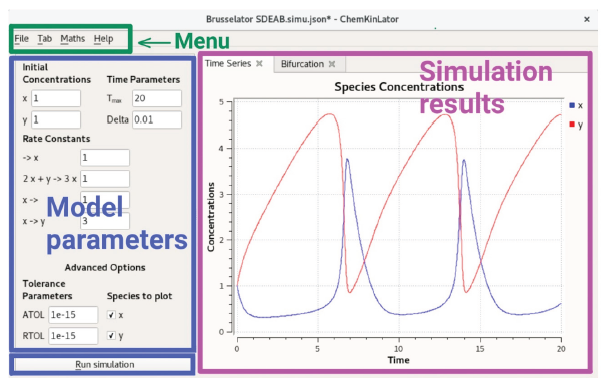
Chemkinlator interface is divided into three different regions, see Figure 1: a menu bar at the top, a column at the left (with the reaction network and parameters needed for the simulation), and a region at the right with the results of a simulation. A button to run a simulation can be found at the bottom of the left column. The region at the right is divided into Tabs. The type of simulation executed depends on the type of the selected Tab. Tabs are of three types: Time Series, Bifurcation, and Flow/Temperature. In the following subsections, we elaborate on each one of the different areas of Chemkinlator.
Menu bar
The Menu bar is composed of four sub-menus:
File: holds all options related to loading, saving, and modifying the current reaction network.
Tab: holds two actions, add a new Tab, and save the data generated by a simulation. Currently, there are two possible Tabs to add: Bifurcation and Flow/Temperature. for the species concentrations, the stoichiometric matrix, and the matrix of reaction orders.
Help: shows basic information about the program, such as license, copyright, and the abbreviations used in the interface.
Model parameters (left column)
The left column contains information about the chemical reaction network and the numerical simulation parameters, which are:
The variable species and their initial concentrations.
The reactions and their rate constants.
The time parameters for simulation: the total time range (Tmax), and the interval between discrete times (Delta).
The tolerance of the convergence, absolute (ATOL), and relative (RTOL), according to the DLSODE routine [18].
The species to plot on the region at the right.
A special region is where the Run simulation button is positioned, the lower part of the left column. Once the Run simulation button is pressed, the simulation specified on the selected Tab at the right (Time Series, Bifurcation, or Flow/Temperature) is run.
A simulation is a solution of the underlying differential equations of the reaction network for each point from time 0 to time Tmax at a user-determined time step, Delta. A simulation can have as many intermediate time steps as one may want. The number of total time steps is limited by the maximum time that we want for the simulation, Tmax.
Simulation results (right region)
The right region contains the results of a simulation. Three types of simulations are possible: Time series, Bifurcation, and Flow/Temperature. Each type of simulation has its Tab type.
A Tab is a self-contained routine that shows the results of performing its specific task, i.e., a Tab is a "blank" space where the results of a simulation will be displayed. What kind of simulation will be shown depends on the type of the Tab. Each Tab is in charge of doing some specific work, a particular simulation, based on the information typed in the left column (the model parameters).
Time series is the main Tab in Chemkinlator. It shows the result of a particular simulation as a function of time, given the parameters introduced in the left column. The Tab showed in Figure 1 is an example of a simulation using the Time series Tab. The Time series Tab does not require additional information other than the values set in the left column.
The Bifurcation Tab requires a short introduction. In the language of dynamical systems, a bifurcation is a change in the qualitative behavior of a system when a parameter is scanned [14, 16]. In Chemkinlator, Bifurcation diagrams are built by simulating a reaction network many times while the value (or values) of a parameter (or a set of parameters) is (are) slightly modified. Thus, each new simulation is slightly different from the one before. Ideally, each simulation is run for a very long time until it reaches a stationary state. After a parameter is scanned, one may see a change in the qualitative behavior of the reaction network, but it could happen that the chosen parameter (or the range where the parameter is scanned) does not produce any change (bifurcation).
One way to test whether a reaction network contains a bifurcation is by exhaustively searching all parameters [8], i.e., run a bifurcation simulation on each one of the parameters and taking the others as constants, and then repeating the process for all the other parameters. The Bifurcation Tab allows the user to scan, also, a combination of rates (a bifurcation as a function of two or more rate constants). In this case, the results could be harder to understand and visualize.
The results of the scan are displayed in a graph as a bifurcation diagram (which may or may not contain a bifurcation, i.e., a change in the qualitative behavior of a system). Figure 2 shows an example of a bifurcation in Brusselator [19, 20], a classical model of chemical oscillations. A bifurcation diagram for the homochirality model of Kondepudi-Nelson [21, 22] is presented in Figure 4.
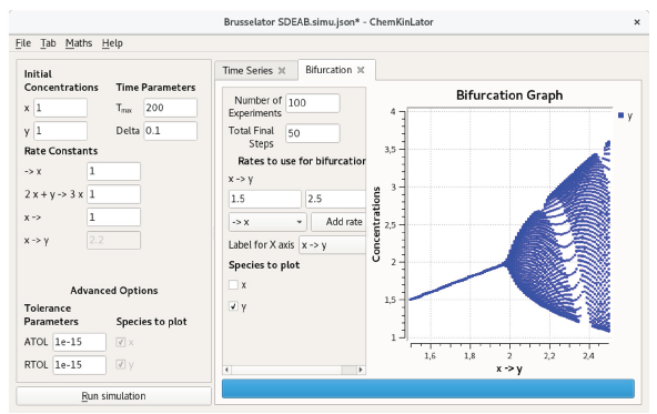
Figure 2 A Chemkinlator simulation example when the Bifurcation Tab was selected: The bifurcation diagram for the Brusselator reaction network [19, 20].
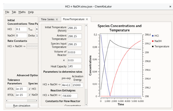
Figure 3 A Chemkinlator simulation example when the Flow/Temperature Tab was selected. Simulation of the acid-base reaction of HC1 with Tris(hydroxymethyl) aminomethane (THAM). This reaction has been used as a calibration reaction for calorimeters [26, 27].
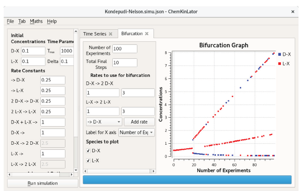
Figure 4 The bifurcation diagram of the Kondepudi-Nelson model, a classical reaction network that generates homochirality. The pitchfork diagram is the result of small noise induced by a floating-point rounding error, causing the concentrations of the enantiomers L and D diverge.
The Bifurcation Tab requires:
The number of experiments to build the bifurcation diagram: Number of Experiments.
The number of final time steps to plot: Total Final Steps. Hopefully, at the end of each simulation, the reaction has found a stationary state.
The rate constant or constants that will be scanned: Rates to use for bifurcation.
The species that will be plotted: Species to plot.
It is possible to create as many independent bifurcation diagrams as one wishes. Each new bifurcation diagram Tab runs independently of all the others. To create a new bifurcation Tab, follow the sequence: Tab > Add Tab > Bifurcation.
The third Tab available in Chemkinlator is the Flow/Temperature Tab. It can simulate a reaction network inside a CSTR. A CSTR reactor vessel implies a perfectly mixed reactor (the composition at any point inside the reaction vessel is the average composition). In a CSTR, the reaction rate at any point will be approximately the same, and the outlet concentration will be identical to the interior composition. Also, the total input volume flow rate is equal to the output volume flow rate, and this is a consequence of the assumption of the homogeneous and constant density of the reaction mixture [23]. Now, the temperature effect, on the reaction mechanism, has been introduced into the reactions rate constants, according to the Arrhenius equation [24]. This temperature effect can be used to simulate a calorimeter that can be adiabatic, pseudo-adiabatic, or flow, depending on heat capacity and global heat transfer constant of the system [25].
The Flow/Temperature Tab requires the following information, see Figure 3:
Initial Temperature in Kelvin.
Ambient Temperature, also in Kelvin.
Reagents temperature at the entrance: Species Input Temperature.
Volume of reactor in dm3.
Global heat transfer constant of the system: k.
Heat capacity of the system: Heat Capacity.
Pre-exponential Factor for the Arrhenius equation, for each reaction.
Activation Energy for each reaction.
Reaction Enthalpies for each reaction.
Reagents input flows: Flow entry.
Concentration of the reagents in reservoirs: Concentration Input.
The International System of Units, SI, was used when the units are not explicit.
A system without input/output flow can be simulated by introducing zero (0) in the Flow entry boxes. An adiabatic calorimeter can be simulated if, additionally to zero flow, the global heat transfer constant is also zero.
Architecture
In this section, we explain the tools used to build Chemkinlator. An in-depth explanation of the inner-workings of the implementation can be found in the documentation which is available with the source code at https://gitlab.com/homochirality/chemkinlator.
Qt 5 [28] was the framework selected to build the user interface. We decided to build the user interface on Qt because it is multi-platform, i.e., only superficial modifications are necessary to make Chemkinlator run in a platform different from the original platform in which it was developed. Chemkinlator was developed in a GNU/Linux environment and required the modification of only one line of code to compile in Windows.
We have chosen C++ [29] as the main language to write Chemkinlator because Qt is written in C++, and the interaction between Qt and C++ is mature. The main routine to simulate a reaction network is written in Fortran 90 (a language optimized for mathematical computations) because an efficient and well-tested Fortran subroutine is used in the core of Chemkinlator: DLSODE [18]. This subroutine is in charge of calculating the species concentrations through time. DLSODE is capable of solving stiff and non-stiff systems offirst-order ordinary differential equations. DLSODE has been thoroughly tested in a multitude of scenarios since its conception in the 1980s. DLSODE is a public domain, and it can be downloaded freely from https://computation.llnl.gov/casc/odepack/odepack_home.html.
Plots and Equations in Chemkinlator are generated using the Qwt library. The Qwt library allows us to produce all plots without any need for external tools, which allows us to offer self-contained binaries that work without any additional software installation.
It is worth noting that a great deal of effort has been put on writing modular code as modular code is easier to extend and maintain. Special effort has been given on making the Tab infrastructure modular. A new Tab (new simulation type) can be added in three steps:
1) Duplicate and rename an old Tab.
2) Connect the new Tab to the program.
3) Configure the building tool to compile the new Tab.
Simulation issues
Floating-point number arithmetic is complicated [30]. It means the operations between real numbers, in a computer, are an approximation because computers can only represent a specific subset of the rational numbers. Computations with floating-point numbers are not always exact, for example, one may expect that the value computed by 0.2 + 0.1 should be the same as 0.3, but this is often not the case; in fact, the computation 0.2 + 0.1 == 0.3 returns false in any programming language where the calculation is performed with floating-point numbers, and the problem worsens as computations compound.
Mathematical simulations and simulators, including Chemkinlator, rely heavily on computations with real/fractional numbers. As a consequence, sometimes a simulation may give an unexpected result, e.g., an unstable reaction network, that was supposed to stay in racemic state given some particular concentration parameters, does not stay in that state [5]. As an example, look at Figure 4, which shows a bifurcation diagram for the Kondepudi-Nelson model [21, 22], a network that generates homochirality. The bifurcation diagram is computed without modifying the initial racemic mixture. For this network (see the particular values included in Figure 4), no change in the concentrations was expected, i.e., we expected to see a single, almost straight line, but instead, we got a "pitchfork" [31]. The central line in the bifurcation diagram indicates all the simulations where the network stayed in a racemic state, which is the expected behavior. The other two indicate all the simulations where the concentrations of the enantiomers diverged, which is unexpected. The reason why many simulations did not stay in the steady-state is the compounding effect of computing over and over with approximated values. Floating-point arithmetic induces a small amount of noise in the simulation, which in this case, is captured by the instability of the reaction network, and it causes the concentrations to diverge.
According to the previous fact, the user may be misguided into thinking that it is worthless to simulate a reaction when the result may be wrong, but that is not the case. Those extreme cases do not occur often in practice, and if they occur, they are not stochastic in nature, i.e., they can be reproduced every time using the same input parameters (initial concentrations, reaction rate constants, etc.). Nonetheless, we ask the user to be suspicious of any weird result. In case the user notices some unexpected result in the computation, we suggest repeating the computation with different parameters to determine whether the cause is related to floating-point arithmetic approximation errors or some other kind of error with the model. Additionally, it is relevant to notice that this kind of situation is always present even in the more sophisticated software.
How to use Chemkinlator: Examples and Applications
In this section, we present the conventions followed by Chemkinlator to input a reaction network. Zero [32], first, second, and third order reactions [33] can be introduced to Chemkinlator through the sequence: File > New reaction network. In Figure 5, it can be seen how to introduce an arbitrary model, including reversible and irreversible reactions.
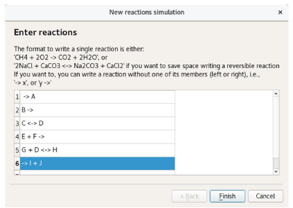
Figure 5 The dialog window to introduce a new reaction network. In this example, an arbitrary set of reactions is introduced.
Chemkinlator reads all reactions as plain text and interprets them in blocks. Chemkinlator first detects whether a reaction is irreversible (->)or reversible (<->), and then it checks for species and their stoichiometric coefficients. Chemkinlator generates automatically the differential equations, the stoichiometric matrix, and the matrix of reaction orders that describe the network.
In Figure 6, a hypothetical network has been introduced to showcase how Chemkinlator can manage zero, first and second-order reactions, together with the parallel, consecutive, and reversible reactions; these are the basic elemental reactions of chemical kinetics [33].
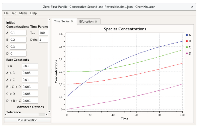
Figure 6 Basic reactions in Chemkinlator: a hypothetical mechanisms base on zero, first, second, consecutive, and parallel elementary reactions [32, 33].
Chemkinlator comes bundled with many examples of simple and complex reactions, including adsorption [34], spontaneous mirror symmetry breaking (homochirality production) [35], and chemical oscillations [36]. Starting from these examples, users can explore a significant part of the chemical kinetics, and anyone can start their particular simulations.
Conclusions
Chemkinlator is a user-friendly tool for chemical kinetics simulations, reliable and well suited for beginners in the field of reaction mechanisms, and which can be of help for advanced users that may need to test chemical mechanisms. Chemkinlator has a simple interface and preloaded examples that help the user to start in silico kinetic studies. Additionally, and for those with more sophisticated requirements, Chemkinlator can also generate bifurcation diagrams, and it is capable of exploring the effects of flows and temperature in reaction networks that occur in a Continuous-flow well-Stirred Tank Reactor (CSTR).
The three types of simulations available in Chemkinlator are conveniently implemented in independent environments, Tab s. Tab s make it easier to change from the basic simulations in the Time series to the more complicated (or complementary) simulations: Bifurcation, or Flow/ Temperature, just by adding a new Tab to do the desired simulation.
The basic and more simple simulations are made in the Time series Tab. The Bifurcation Tab allows to explore the complexity of a model as a function of one or more of their rate constants; and the Flow/Temperature studies the effect of flows in a CSTR and the effect of temperature on the kinetic rate constants according to the Arrhenius equation, which allows to simulate adiabatic, pseudo-adiabatic and flow calorimeters.
Chemkinlator is free software and can be extended by adding new Tab s. We encourage developers and chemists alike to check the main web page for more information on how to use it and how to add new Tab s and simulations.

