English (pdf)
 Article in xml format
 Article references
 Send this article by e-mail
 Cited by SciELO
  Cited by Google
  Similars in
SciELO
Similars in
SciELO  Similars in Google
 Permalink
INTRODUCTION
Nowadays there are studies of causality between Producer Price Index, (henceforth PPI); and Consumer Price Index, (henceforth CPI). But making an investigation to analyze the relation between those two indexes in South America, is innovative. In order to contextualize, the CPI represents the cost of living (Selçuk, 2011). CPI is also consider as an important economic indicator in any country as it provides temporarily data of the prices paid by urban consumers for a representative goods and services basket (Mel, 2011).
The CPI examines the average behavior of prices from a basket that contains goods and services, such as food, transportation, medical care, housing and education. The fundamental objective of the CPI is to identify the evolution of the prices of various goods and services of a representative hamper of national consumption. Besides, the CPI is calculated by taking price changes from each item in the predetermined basket of goods and services. For example, in the United States the major indexes of the seven points of goods, are food, wine and drinks house, dress, traffic, medical health, entertainment, among others (Mel, 2011).
On the other hand, Producer Price Index measures the rate of change in prices of products sold as they leave the producers. They exclude any taxes, transport and trade margins that the purchaser may have to pay (OECD, 2017). The PPI is an index that captures the prices average variation of goods offered inside of a country, that is, as much produced and consumed internally as imported. It is important to clarify that the basket of goods is different for the CPI on each country, which means that CPI is not suitable to compare between countries.
All kinds of results have been found, from the PPI is an anticipated indicator of the CPI, to they are coincident indicators, that the CPI leads the PPI. The PPI is the indicator that precedes the CPI in the market chain, since production is prior to consumption. According to Martínez, Caicedo and Tique (2012), the main explanations for the differences in the performance of the PPI and the CPI have been price controls, demand and supply factors, adjustments in marketing margins, as well as differentials in the transmission of the exchange rate, among others; without emphasizing the differences of methodological cutting existing between the two hampers.
On this text we tried to decide the relationship between PPI and CPI for six countries in South America (Brazil, Colombia, Ecuador, Paraguay and Uruguay). To decide this relation the method VAR o VEC is established, depending on the case, which establishes the dependency or independence between those establishes variables, following the stages of identification, estimation and validation of the model. In addition, the impulse response function is estimated. Finally, if it is found a causality between those variables it can be decide with a structural model, the causality through time can be proved by evidences of causality, which also can help to establish the endogeneity of VAR or VEC variables. On that case, it will be developed through Toda and Tamamoto test, which also decide the relation between stationary variables, as it is on the case of Granger (1969), but also between non-stationary variables. The data's periodicity is annual, and periods of time vary between countries, depending on own behavior of the CPI and PPI to country.
The document is organized in five parts. The first is the introduction; in the second, some previous studies are reviewed; subsequently the methodology is exposed; in the fourth section the results are analyzed, and finally the conclusions are referred.
PREVIOUS RESEARCH
Causality between CPI and PPI has been investigated in different countries around the world but there are not many studies related to the analysis of these two variables in South American countries.
The Faculty of Economics and Administrative Sciences in the Afyon Kocatepe University (Selçuk, 2011) carried out a study to examine the causal relationship between PPI and CPI for five selected European countries, Germany, France, Sweden, Finland and Netherlands. The author (2011) uses the analysis of cointegration and Granger's causality developed by Toda and Yamamoto to determine if there is a causal relationship between the PPI and the CPI of the five selected European countries. According to the results of the cointegration test of Johansen and Juselius (1990), the author finds cointegration between the two variables only in Germany, while in the other countries analyzed the series are not cointegrated. The results of Toda and Yamamoto causality test show the existence of a unidirectional causal relationship of the PPI to the CPI, in Finland and France. In Germany, there is evidence of a bidirectional causality between the PPI and the CPI. Finally, no significant causality was detected in the Netherlands and Sweden.
Furthermore, Bryan, Cecchetti and Wiggins (2011) executed an investigation which was name Efficient Inflation Estimation, "this paper investigates the use of trimmed means as high-frequency estimators of inflation". The known characteristics of price change distributions, specifically the observation "that they generally exhibit high levels of kurtosis, imply that simple averages of price data are unlikely to produce efficient estimates of inflation". They find that trimming 9 % from each tail of the CPI price-change distribution from the tails of the PPI price-change distribution, yields an efficient estimator of core inflation "for these two series, although lesser trims also produce substantial efficiency gains. Historically the optimal trimmed estimators are found to be nearly 23 % more efficient" (Bryan et al., 2011, p. 1).
Nader Hakimipoor carried out an investigation named "Investigation on Causality Relationship between Consumer Price Index and Producer Price Index in Iran''. The aim was to investigate the relationship between Consumer Price Index (CPI) and Producer Price Index (PPI) in Iran by using monthly data from 2010-2011. The result of Johansen's co-integration test indicated that there is no long-run relationship between these series; therefore, there is no causality relationship between them in the long-run. On the other side, the results indicate that there is bidirectional causality between two indices in short-run (Hakimipoor, 2016).
"Explorando la relación entre el IPC e IPP: el caso colombiano" was named an study that was accomplished in Colombia and it was found that the PPI anticipates the CPI, and depending on the analyzed group, the leadership of the IPP may, by one or even several months, anticipates the CPI. These findings are clearly useful as input to improve forecasting models of inflation and consumer decisions of the monetary authority (Martínez et al., 2012).
Other study on Colombia was named "Relación entre el índice de precios del productor (IPP) y el índice de precios al consumidor (IPC)'', and this study gives relative information that according to the econometric techniques used, no evidence was found of a relationship between the annual variations of total CPI and total CPI. This would imply that contrary to what has been believed in Colombia, the IPP would not be a leading indicator of the CPI. However, by extracting non-common groupings (services in the IPC and the intermediate consumption in the IPP), the series presented a long link term (cointegrated), and causal relations occurred in both directions (Campos & Jalil, 2000).
Reviewing the most recent researches about the topic, it is observed that there is no convincing evidence of the direction of causality between the CPI and the PPI, in different countries. However, a large part of the studies show a causality of the PPI towards the CPI.
The contribution of this paper to the existing literature is that few studies contrast the relationship of these two variables to different countries, especially on South American region, where the principal problem to estimate the time series models is to get the variables with considerable period of time for the variables.
METHODOLOGY
It is also important to highlight that in the data collected the rank of years is different for the selected South American countries. Both CPI and PPI data were obtained from World Bank Data and there was not enough information. The countries with the corresponding rank of age in studies are: Brazil (1996-2015), Colombia (1980-2015), Ecuador (19982015), Paraguay (1996-2015), Peru (1992-2015) and Uruguay (1990-2015); the data's periodicity is annual. The rest of the South American countries do not have enough information for the analysis. In order to carry out the model it was necessary the program Eviews 9, which is used to analyze time series variables. The data from these data bases are on percentages.
VAR methodology, proposed by Sims (1980), alternately a simultaneous equations system where all the variables are considered endogenous, due to all the variables are explain by their own lags and the lags of the other system variables. The VAR and VEC model are intended to clarify the dynamic relationship that may exist between different time series and show the possible behavior of the series against specific perturbations of some variable (s).
The first step to apply the VAR models is that the variables are stationary, thus, their means and variances are constant over time, or non-stationary, in the case of applying a VEC model. The stationarity is tested through the Augmented Dickey-Fuller Unitary Root Test (1979) and the Schwarz (1978) information criterion. Subsequently, in the case of non-stationary variables, the Johansen and Juselius cointegration test (1990), with the purpose of determining whether the combination of non-stationary series results in a stationary series, that is, if the non-stationary series are cointegrated. When the series are integrated, a VEC model is applied.
Once it is determined the type of model to apply, based on the information criteria of Akaike, Schwartz and Han-nan-Quinn (1979), set the order of the autoregressive vector or the number of lags to include, for each of the countries. Later, to be sure of the stability of this model it is used the portmanteau test. This test evidences that the model does not have residual autocorrelation up to lag. In order to confirm the results, we used the graphic method. It is necessary to confirm that the value does not exceed one and the way how this is done is through the table method. Finally, it has been determined that the model analyzed is stable. After having examined the stability of the model, the following step is to impulse the model so as to analyze the response to Cholesky between the variables; that is to say, the IPP response to IPC shocks is analyzed, and in the opposite direction, in each of the countries.
Finally, to determine if causality exists between the variables, the test Toda and Yamamoto will be estimated, due to the fact that is the standard Granger (1969) causality test for inferring leads and lags among integrated variables is likely to give spurious regression results and F-test becomes invalid unless the variables are co-integrated.
Toda and Yamamoto's method has more advantages that it does not matter whether series are I (0), I (1), I (2) even if the series are co-integrated. Also, Toda and Yamamoto can be applied when there is no integration or stability and when the Rank condition is not satisfied (Selçuk, 2011). Unlike the conventional Granger causality test, the Toda and Yamamoto (1995) approach fits a standard vector auto-regression on levels of the variables is not on the first difference of the variables (Selçuk, 2011).
Autoregressive models are used when there is more than one dependent variable. They are the most suitable models to model stationary time series, because in general, they perform better than univariate models. An advantage of these models is that you do not need to differentiate between endogenous and exogenous variables, since they all become endogenous, that is, they avoid the problems that exist due to endogeneity. Another advantage is that VAR models are usually better than traditional ARIMA, ARMA models. In addition, according to the literature review, the use of this type of models to determine relationships between the CPI and the IPP is growing.
EMPIRICAL RESULTS
CPI and PPI behavior
Brazil is one of the main countries of South America. The rate of inflation in Brazil during the study period (19962015) has shown a relatively stable behavior, however, according to the Banco Central do Brasil (2016), inflation in Brazil closed in 2015 at its highest level in more than 12 years, exceeding 10 %, at a time when the main economy of Latin America faces a deep recession. The increase in taxes, the high public spending and the climatic phenomenon of "El Niño" are aspects that explain the growing inflation.
Colombia is one of the few countries in Latin America that recorded a decreasing behavior of the inflation rate during the period studied (1980-2015). The highest levels of inflation occurred in 1991, with inflation above 30 %, due to the process of economic opening experienced by this country. On the other hand, the lowest inflation rate was recorded in 2013, mainly explained by the lower increase in food group prices.
In Peru, since the implementation of the inflation explicit targeting scheme in 2002, an average annual inflation of 2.9 % was reached, the lowest among the countries that follow the same scheme in Latin America. According to the study period (1992-2015), before 1996, inflation reached double-digit rates; but after 1997 there was a decreasing trend in prices, which has allowed achieving macroeconomic stability and promoting economic growth.
One of the main inflationary processes in Ecuador began in 2000 when the dollarization system was applied in the national economy, being one of the few countries to apply this system in Latin America. Dollarization allowed Ecuador to reduce inflation to one-digit figures but not in the short term, since the year 2000 ended with inflation above 90 %, mainly due to the lag of the 1999 crisis and the adjustment of the new system of dollarization. As of 2013, inflation begins a significant deceleration until reaching levels of 2 %.
Paraguay is one of the few countries in South America that registers high rates of GDP growth in the last 20 years, which is reflected in a good effectiveness in controlling inflation. At the end of 1995, cumulative inflation was in the order of 10 %, but it quickly began to fall to reach one-digit rates, especially from 2005-2006 when the Central Bank adopted a new monetary policy framework based on inflation goals. In 2015, inflation reached 3.1 %, measured through the CPI variation, being the lowest in recent years. The reduction in inflation in recent years has been accompanied by a trend of appreciation of the Guaraní.
Uruguay is one of the countries with the highest inflation rates in the region, in 2015 inflation was 9.4 %, the highest in the last 12 years, after which in 2002 it will reach a rate of 25.9 %. A growing fiscal deficit, the depreciation of the domestic currency against the dollar and a significant wage imbalance between the public and private sectors, explain in greater proportion the behavior of inflation.
At general level, it would be expected the slowdown in growth in China and the continuous fall in the prices of crude oil and other raw materials, reduce the inflation rates of most countries in the region, and in fact happens in most countries, however, countries such as Brazil, which is China's main trading partner in South America, registers rising figures of inflation.
Econometric Estimates
In Annex 1, both PPI and CPI were plotted at levels (based on 2010) for each of the countries, according to the availability of data with which they were found. In general terms, it is observed that both the CPI and IPP show an increasing tendency with respect to the time, which is logical taking into account the naturalness of the variables.
As evidenced by the graphs in Annex 1, there is a great similarity between the two series, mainly explained, because in the short term there is the transfer of the price between producer and consumer, mostly in perishable agricultural goods, because of the nature of the product, if it is not commercialized, in the short term the farmer would lose all the product. In the case of non-perishables, prices are affected by abundance or scarcity of their raw material, since the consumer can substitute a processed product for a natural one if the price is favorable. This information is the first indication of non-stationarity.
At the beginning of the analysis, it is used the unit root test of Augmented Dickey-Fuller (ADF) that is employed to test the stationary of the series. In the Table 1 the results of the unit root test for the countries under study are shown. This table reveals that we cannot accept the alternative hypothesis of unit roots for variables in levels, for all the countries studied, both the CPI and the PPI were non-stationary1, with the exception of Brazil, Peru and Uruguay, where the growth of the CPI and IPP was estimated and in both cases they were stationary2. On the other hand, the CPI and the PPI of Colombia, Ecuador and Paraguay, the set of variables turned out to be stationary.
Table 1 Summary unit root test of Augmented Dickey-Fuller (ADF).
* MacKinnon (19596) one-sided p-values. ** In these countries the growth rates of the CPI and the PPI are estimated, unlike the other countries, for which these variables were estimated in levels.
Source: EViews, Own calculations 1.
Once the stationarity of the series is identified, the next step is to select the number of optimal lags for model estimation. In this case, the procedure was used of EViews "Lag Order Selection Criteria", which calculates the optimal lag from statistics known as information criteria such as the Akaike, Schwarz y Hannan-Quinn. From a VAR (p) representation in rty levels, the number of relevant lags for each country was selected; in Brazil were established 1 lags, VAR(1), in Colombia VAR(2), Ecuador VAR(2), Peru VAR(2), Paraguay VAR(2) y Uruguay VAR(2). According to Lütkepohl (2004) and Espinosa y Vaca (2015), VAR (p) Model can be written as a VEC model (p-1), that is, the Error Correction Model is of order p-1. In this case, a VEC model (1) was estimated for Colombia, and a VEC (1) for Ecuador and Paraguay; for Brazil a VAR (1) was estimated and for Peru and Uruguay a VAR (2).
The next step is to estimate the test of Johansen and Juselius (1990), which allows to determine if the series are cointegrated if a cointegration relationship exists, there is necessarily a representation of this long-term relationship in a short term that corrects the error and prevents the cointegrated series are dispersed over time (Loria, 2007A necessary condition to apply the test of cointegration is that the variables are integrated of the same order, therefore the Table 2 shows the test of Johansen and Juselius (1990) for Colombia, Ecuador and Paraguay.
For Colombia a model with a quadratic tendency and intercept was utilized; in Ecuador, a model without trend or intercept was applied, while in Paraguay was a model with no linear trend in the data of the cointegration equation but with intercept. The results indicate the presence of a cointegrating vector between the series according to the statistic of the trace and the statistic of the maximum own value to 5 % of significance. Therefore, there can only be a cointegration relation with two variables. It is concluded that there is a long-term stationary relationship between the CPI and the PPI in the three countries analyzed.
VEC models differ from VAR in that employ non-estationary variables, and in this sense is able to capture elements of great importance in the analysis of economic time series (Bonilla, 2011). Formally, VAR(p) and VEC(p) models are defined below:
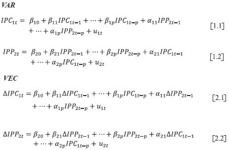
Where in the VEC model the dependent variable in each equation is the first difference of the corresponding variable, either or , expressed as a function of its own differences lags, the lags of the other variable in difference and the term of lagging cointegration. The VAR model, on the other hand, is estimated taking into account the variables in levels. Tables 3 y 4 show the estimation of the VAR and VEC models according to the characteristics of each of the countries studied.
Table 3 VAR Model estimated by countries.
Source: EViews, Own calculations 3, Standard error in (), t-statistics in []Own calculations.
Table 4 VEC model estimated by country.
Source: EViews, Own calculations 4, Standard error in (), t-statistics in []Own calculations.
In the case of Peru, Colombia and Paraguay, the results of the model allow to conclude that the variation of the PPI explains negatively the variation of the CPI. On the other hand, in Peru and Colombia it was also found that the variation of the CPI explains positively the variation of the PPI. In contrast, in Brazil and Ecuador it was found that the variation of the CPI explains negatively the variation of the PPI. Only in Peru the CPI explains the PPI and in the opposite direction. Finally, it was found that in Uruguay the CPI explains the variation from PPI and of itself, also the PPI explains the variation of CPI and of itself.
With the purpose of determining the causal relationship between the CPI and the IPP for the different countries studied, it was made the Toda and Yamamoto test with the lag length selected (k), VEC order (k+dmax), MWald statistics, p values and the direction of causality.
On the causality test of Toda and Yamamoto (1995), as it is explained on Frimpong and Oteng-Abayie (2008), it is not important the integration order of the variables, or if the variables are cointegrades or not, unlike Granger (1969) and Sims (1972) where the variables to analyze have to be estationaries, therefore only applicable to VAR models. But when the variables are not stationary but are cointegrated a VEC model is applied, in which case, Granger or Sims would not determine if there is causal relationship, so the literature recommends applying the Toda and Yamamoto test (see Table 5).
Table 5 Toda-Yamamoto No-Causality Test Results.
Notes: ***, **, * denotes 1 %, 5 %, and 10 % significance level, respectively.
Source: Own calculation 5.
Next, we will try to determine if there is causality between the past of the consumer price index and the producer price index, likewise, causality is evaluated in the opposite direction by contrasting the past of the producer price index with the consumer price index. Therefore, if in either or both relations makes sense, means that the past of one variable affects the present of another.
In Peru, this result indicates that there is bidirectional causality between PPI and CPI; for this reason, it can have concluded supported by the empirical evidence, that the implication can predict the inflation by using the PPI in Peru, and predicts the price of producing by using the inflation. On the other hand, in Paraguay it is possible to predict the PPI due to the inflation. In the rest of the studied countries (Brazil, Colombia, Ecuador and Uruguay) there is no significant causality between PPI and CPI.
Due to the fact that in Brazil, Colombia, Ecuador and Uruguay no causality was found in any of the senses, it was not possible to detect a long-term relationship between the CPI and the PPI, therefore, an increase or decrease in either of the two indicators do not affect the behavior of the other.
In the case of Peru and Paraguay, where there is evidence of causality, IPP leads the IPC, given the greater tradability of the PPI and its greater sensitivity and response to fluctuations in international prices of food and raw materials, and exchange rate.
The estimates made for the different countries are not conclusive, because of it is important to bear in mind that the two baskets of prices analyzed are widely different by size, coverage, location in the marketing chain, origin and structure of the weights, tradability, composition, etc. In addition, according to economic, social and cultural characteristics, each country has a different consumption basket. These conceptual and methodological differences hinder the comparison of the two indices, because of as was proven in most of the countries studied, there was no type of leadership or long-term relationship between them; this result is common in different studies conducted on the subject.
The next step on this paper is analyzing the effect caused by the other variables that were not taken into account in the model. So, for this reason, it was applied the method of response by Cholesky on S.D for each country under study.
The Figure 1, of the impulse-response function, allows establishing more precisely what is the effect caused in the CPI due to a shock in the IPP, and in the opposite direction.

In Brazil, both the CPI and the IPP, measured in growth rates, respond to shocks both in itself and in the other variable, where its impact disappears after approximately six periods.
When examining the impulse response effect for ten months, it is observed that the response of the IPP to a shock in itself is positive, 6.51 % for period one and 2.19 % for period two, however, the effect is diluted by the sixth month. For its part, the effect of IPP on CPI is negative, for the first period is zero, but for the second and third is 0.69 % and 0.34 % respectively, which also disappears around the sixth month.
A CPI shock also has greater effects on itself, but only during the first period, and from the second period, the CPI has a greater impact on the PPI. In both cases the effect decreases in period six and tends to zero.
Figure 3 shows, both the CPI and the IPP of Colombia, measured in levels, which respond to shocks both in itself and in the other variable, where its impact stabilizes around month six. Specifically, a shock in the PPI generates a greater impact in itself as an increase of 3.72 % for the first period, 2.06 % in the second, then stabilized at 1.54 % from the seventh period. The impact of a shock on the PPI in the CPI is also positive, but is relatively smaller; for the second period is 0.78 %, while for the third and fourth periods it is 0.73 % and 0.78 %, respectively.
On the other hand, a shock in the CPI has greater effects on the PPI than on itself. The IPP's response to changes in the PPI stabilized around the sixth month by approximately 2.6 %. In both cases, the effect does not disappear in the long term. In Colombia, IPP shocks, such as IPP shocks, generate permanent increases in themselves and on the other variable, so that, given these changes, the variables will not return to their initial values.
A shock in the IPP generates a greater effect in itself, as it causes an increase of 14.31 % for the first period, 10.75 % in the second, then, after the sixth month, retains a value close to 10.3 %. On the contrary, the impact of a change in the PPI leads to a negative impact on the CPI, for the second period is -5.67 %, while for the third and fourth periods it is -4.81 % and -5 %, respectively. After period six, the effect becomes permanent with a negative close to 5.2 %.
On the other hand, a shock in the CPI shows greater effects on the PPI than on itself during the first period, like Colombia. From the second period, the CPI reacts with greater proportion than the IPP. A change in the CPI generates permanent changes in the PPI after ten months, where it retains a value close to 0.24 %. A change in the CPI generates, until the fourth month, positive effects on itself, but from the fifth month this trend becomes negative until stabilizing around -0.12 %. In both cases, the effect does not disappear in the long term, so, given these changes, the variables will not return to their initial values.
In Peru, both the CPI and the PPI, measured in growth rate, respond to shocks both in itself and in the other variable, where its impact is transient because the effect disappears after approximately seven months. In assessing the response of the IPP to a shock in itself, which is the largest, an increase is seen in the variation of the PPI during the first month, for the second and third month a reduction in the PPI is indicated, in the fourth and fifth month there is an increase in the index, but not of the same magnitude of the previous months, on this way the shock is diluted and by the month twelve the shocks disappear.
The impact of a CPI shock on the PPI is similar to the previous one, in the first and second month the impact is positive, 1.20 % and 0.35 % respectively, while in the period three and four the impact becomes negative, -0.30 % and 0.001 % respectively, in the two following periods the impact returns to be positive, and in the following months returns to be negative. And until the month in which the effect of CPI on the PPI in Peru is diluted. The results are indicated in Figure 4.
In Paraguay, the CPI and IPP measures in levels, as in Colombia, it responds to shocks both in itself and in the other variable, where its impact continues to spread in the long run. A shock in the CPI generates a greater impact in itself by producing an increase of 2.23 % for the first period and 2.51 % in the second; the impact continues to grow over time. The impact that a shock on the CPI generates in the PPI is also positive and increasing, although proportionally lower compared to the CPI response, for the third month is 0.44 % while for the fourth and fifth month it is 1.24 % and 2.10 %, respectively.
On the other hand, a shock in the PPI generates a greater impact on the CPI than on itself. In both cases, the effect does not disappear in the long term; both the IPP shocks and the IPP shocks generate permanent increases in themselves and on the other variable. So that, given these changes, the variables will not return to their initial values. The results are indicated in Figure 5.
Finally, in Uruguay, both CPI and PPI are in growth rate, they respond to shocks both in itself and in the other variable, where its impact disappears after approximately twelve months (see Figure 6).

When examining the impulse response effect, it is observed that the response of the IPP to a shock in itself is positive, 4.94 % para el period one and 0.88 % for the period two; in periods three, four and five the response of the IPP becomes negative, and in this way it oscillates until the effect is diluted by the fourteenth month. On the other hand, the effect of IPP on CPI is greater, for the first period is 6.66 %, while for the second and third it is 5.75 % and 0.33 % respectively, then the response becomes negative during the next two months, and then respond positively until it disappears around month fourteen.
A CPI shock has greater effects on the PPI, 4.07 %, 2.84 % and 1.24 % during the first three months respectively. The effect is diluted around month fourteen. This effect is common in Brazil and Peru, where a VAR model was also applied.
Finally, after the estimation of the models by country, to validate the models the behavior of the residuals in each one of the applied models was analyzed to verify that they fulfilled the assumptions that are made in this features, that is a behave white noise.
The first thing that was done was the analysis of unit roots (see Annex 2), where you can see, for the different countries, that all eigenvalues of the autoregressive polynomial of VAR and VEC are less than one, and for this reason it is concluded that the system satisfies the conditions of stability and seasonality.
The normality of the residues for each of the models was contrasted by the Cholesky test, which defines as null hypothesis the existence normality in the model, and as an alternative hypothesis the non-existence of normality in the model. Annex 3 includes the results of Cholesky's normality test, which concludes that in each of the models for the different countries, the null hypothesis is accepted since the parameters of symmetry and kurtosis are considered in the Jarque-Bera test which indicates that the model in the joint test has a probability greater than 0.05.
A very important test with respect to the residuals in the VAR and VEC models is the autocorrelation. Therefore, we performed the Portmanteau test and the LM (Lagrange multipliers) test for serial correlation of the residuals, which check whether any autocorrelation, within a group of autocorrelations of the residual time series is different of zero. The results are shown in Annex 4. In all countries, evidence indicates that there is no autocorrelation in residuals; therefore, it is white noise.
Finally, to determine the presence of heteroscedasticity the probability of the joint test was analyzed, where it is considered as a null hypothesis that the variance of the errors is homoscedastic, and alternatively, that the variance of the errors is heteroscedastic. Annex 5 shows the estimates; from which it is concluded that in all countries the residual estimator models are homoscedastic.
CONCLUSIONS
The CPI and IPP are two key indicators for determining price changes in any world economy, which have different approaches in terms of composition and economic approach. Despite this, it is observed that both indicators show sensitivity to sudden shocks both in themselves and in the other variable, effect that varies depending on the characteristics of each country.
For this study, cointegration and methodology of Granger no-causality test developed by Toda and Yamamoto, are applied to investigate the causality between PPI and CPI for the selected South American countries, using annual data. As it was determined that in Brazil, Peru and Uruguay there is a long-term cointegration relationship, but not co-integra0ted in Colombia, Ecuador and Paraguay.
According to the econometric techniques carried out, no empirical evidence was found of a relationship between the annual variations of the CPI and the PPI for Brazil, Colombia, Ecuador and Uruguay; this would imply that contrary to what has been believed, the PPI would not be a leader indicator of the CPI.
On the other part of the study, the results of Toda and Yamamoto no-causality test indicate bidirectional causality between CPI and PPI in Peru, and for Paraguay was detected a causality from CPI to PPI. In the case of Brazil, Colombia, Ecuador and Uruguay there is no significant evidence to ensure a causality between these variables.
It is important to comment that the results in the direction of causality between CPI and PPI for the different countries analyzed can be explained mainly by the differences in the content of the hamper of goods and services that are used to estimate the producer price indices and the consumer. In addition, important variables can be omitted for the model.
The main explanations by which the CPI and the PPI do not have a statistical relationship are the different price controls, the mismatches in marketing margins, the differences in the transmission of the exchange rate, among others.
The relationship between the CPI and the PPI was estimated for six South American countries, where three VAR models (Brazil, Peru and Uruguay) and three VEC models were applied (Colombia, Ecuador and Paraguay) which depend on the cointegration of the series studied. From the estimation of the models of Peru, Colombia and Paraguay shows a negative effect of IPP on the CPI. Similarly, in Brazil and Ecuador, a negative effect of the CPI on the IPP.
A common result in the estimated VAR models, that in the impulse response function, after a shock of the CPI and/ or the PPI on the other variable and on itself, the effects disappear in time and the variables return to their original values.
In the VEC models, after a shock of the CPI and/or the PPI on the other variable and on itself, the effects do not disappear over time; therefore the variables present permanent changes in the time.
One of the biggest limitations when carrying out this analysis is related to the data, no data availability was found for the same periods of time in all countries, hence different periods are taken for most countries. The periodicity was also affected, because of long series of time are not available. This considerably limits the results to the extent that effects cannot be captured by the variables in the long term. Limiting data can lead to biases or behaviors that are not explained, like happened in most countries.
It requires a greater effort on the part of the statistical organisms of the Latin American countries to build longer historical statistical series that allow making more reliable and true analyzes, with the consequent benefit for the policymakers of having reliable information. Likewise, it is necessary to unify methodological criteria for the calculation of the PPI and the CPI, with the purpose of making these variables comparable between countries.
Analyzes are recommended for future studies to make out between the CPI and the PPI with a more disaggregated level of detail, which allows comparing the group of goods within the consumption hampers, and enables a higher degree of comparability between countries.