João Correia Leite**

* I would like to thank Dr. Maurizio Zanardi and Dr. Hernán Vallejo for their guidance and support during the development of this paper. I gratefullyacknowledge the financial support from the International Office of Tilburg University for my stay in Colombia.

** Email: joao_mcleite@hotmail.com.

This article was received December 13th 2007, modified May 20th 2008, and finally accepted June 9th 2008.

Abstract

This thesis makes use of the gravity model to analyze the effectiveness of EU's consecutive GSP programs on promoting Colombian exports. It concludes that the European preference systems have been consecutively less effective on boosting Colombian exports over time. This is explained by three major factors: an increasingly more efficient US preference system; a deepening of the Andean integration; and occurrence of EU enlargements. The sectoral analysis reveals that the GSP program of the EU had different effects across sectors.

Key words: gravity model, Colombia, European Union, GSP, trade.

JEL Classification: F1.

Resumen

Este trabajo hace uso del modelo gravitacional para analizar la eficacia de los consecutivos sistemas de preferencia de la Unión Europea (UU. EE.) en promover las exportaciones Colombianas. El estudio concluye que las preferencias concedidas por la UU. EE. han sido consecutivamente menos eficaces en la promoción de las exportaciones Colombianas. Este facto es explicado por tres factores: un sistema de preferencias de EE. UU. consecutivamente más eficiente; el profundizar de la integración Andina; y la ocurrencia de expansiones de la UU. EE. Además, el análisis sectorial revela que el programa europeo ha tenido diferentes efectos en diferentes sectores de exportaciones.

Palabras clave: modelo gravitacional, Colombia, GSP, comercio.

Clasificación JEL: F1.

Introduction

Colombia will soon start negotiations with the EU concerning the trade relations between these two economic areas. At stake is the achievement of an agreement which could allow for a further reduction of the trade barriers still in place among these economies. In the EC's words "[FTAs] are part of our negotiations for […] future association agreements with Central America and the Andean Community" (EC, 2006: 10). But the establishment of FTAs is not the only mechanism through which countries facilitate trade flows. For several decades developed countries have granted a special treatment to the exports of their developing counterparts under a scheme known as the Generalized System of Preferences (GSP).

Colombian exports to the EU market have been subject to GSP treatment since 1971. This system makes Colombian (and many other developing countries') exports to the EU subject to lower import tariffs than those applied on a most favoured nation (MFN) basis. The GSP is mostly considered to have a positive impact over the exports of the countries that benefit from it. Nevertheless, its true impact over Colombian exports remains unknown. Furthermore, it is unclear weather the effectiveness of this program on promoting exports has increased throughout time. In a time where Colombia and the EU are willing to deepen their trade ties, it becomes extremely relevant to understand which role the GSP has played on influencing the flow of goods between them.

This paper presents an empirical analysis of the effectiveness of EU's GSP program on promoting Colombian exports. It will specially focus on trying to understand whether this GSP program was progressively more/less successful during the period under analysis (1991-2005). In order to do so, it has to take into account the global framework of Colombian trade relations. For this reason, it explores the evolution of Colombian exports to a set of 167 countries taking into consideration the most relevant trade agreements in place between these countries and Colombia. Besides that, this thesis puts Colombia at the center of the analysis. While other studies explore the development of Colombian trade flows taking into account world patterns, this paper estimates the determinants of Colombian trade flows by using a gravity model specific to its exports. By taking into account Colombian trade patterns as the basis of the analysis it is possible to correctly estimate the effects of the policies under study. In addition, while other studies take the different GSPs applied throughout the years as a single program, this paper disaggregates the consecutive GSP programs applied by the EU to Colombia with the objective of understanding whether its effectiveness increased/decreased.

Section I presents the most relevant trade relations between Colombia and its partners. Section II shows the theoretical foundations of the model to be used: the gravity equation. Section III describes the model and motivates the estimation methodology to be used. Section IV presents and discusses the results of the empirical analysis. Section V presents the summary of conclusions, contributions and suggestions for further research.

I. Colombian trade relations

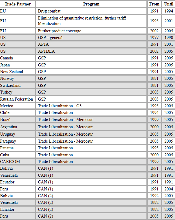
Colombia is a very interesting case in what concerns its institutional relations concerning international trade. It is a GATT/WTO member since 1981. Its main trade partners are, according to 2005 figures, the US, the EU, Venezuela, Ecuador, Peru, Mexico and other Latin American countries. It has several formal trade arrangements. It forms a free trade area with Bolivia, Venezuela, Ecuador and Peru in the framework of the Andean Community (CAN, from Spanish Comunidad Andina de Naciones). Under the economic integration scheme set by the Group of Three (G3 - Colombia, Mexico and Venezuela), Colombian exports enjoy tariff reductions in Mexico. Under some kind of trade liberalization schemes its exports also enjoy tariff reductions in the Mercosur member countries (Brazil, Argentina, Uruguay and Paraguay) and Chile, among others. Its exports are subject to a special treatment under preferential systems in the EU, US, Canada, Japan, New Zealand, Norway, Russian Federation, Turkey and Switzerland. Besides that, it has lately been negotiating the formation of free trade areas with some of its main trade partners (of which the FTA with the US is the most relevant). This by itself explains the complexity of the framework in which Colombian trade is based on (see Table A1 in the Appendix). In the rest of this section the preferential systems applied by the EU and the US are introduced and the Colombian exports are analyzed in detail.

A. The GSP of the EU

In 1990 a new special arrangement supporting measures to combat drugs was granted by the EU to the countries of the Andean Community (among which Colombia) on the basis that their development was being seriously threatened by drug production and traffic activities in place in these countries. This regime intended to create special export opportunities that would substitute crop production in a way of promoting social and economic development in those countries. This regime extended duty-free access for a broad range of products.

In 1995 a new framework was implemented. While the traditional goal of promoting economic development among the target countries was maintained, its interpretation was modified. In order to promote a sustainable development among the beneficiary countries, special incentives related to environmental protection and the respect for social rights were introduced. One of the most relevant features of this new framework was the elimination of all quantitative restrictions (such as quotas). The products began being classified in four different categories with progressive tariff reductions according to their sensitivity.

The introduction of a safeguard clause determined that GSP preferences might be suspended for certain products originating from certain countries in the event that those imports cause or threaten to cause serious difficulties to a EU producer. This raises a serious question of commitment by the EU in conceding these preferences. If following a certain investment a Colombian producer would succeed in increasing its exports to the EU market in such a way that it actually hinder EU producers, the GSP concessions might be withdrawn. This possibility will hold back producer from investing in the first place, which clearly goes against the program primary goal of sustainable development.

In 2002 the EU revised the framework introduced in 1995. The special arrangements to combat drug production and traffic provided further product coverage in terms of duty-free access. This led to a complete suspension of duties applicable to agricultural and industrial products imported from Colombia.

Looking through period under analysis (1991 – 2005) it is easy to identify 3 different GSP schemes applied to Colombia by the EU: the special arrangement to combat drugs was in place since 1991; in 1995 all quantitative restrictions were eliminated and progressive tariff reductions were applied according to the sensitivity of the products; finally in 2002 the preferential product coverage was enlarged. It is relevant to say that, according to the EC, the utilisation ratio of the GSP program by the Andean countries (among which Colombia) increased in the considered period reaching 88% in 2003, a significantly high value when compared with the 50% average for all GSP beneficiaries.

B. The GSP of the US

Among the remaining GSP schemes applied to Colombia, the one extended by the US deserves special attention. Besides being the most important Colombian trade partner, the US also introduced new frameworks of preferences during the period in analysis.

In 1991 the Andean Trade Preference Act (APTA) was approved by the US government as part of the fight against drug trafficking. This program intended to create viable legal alternatives to crop producers through the elimination of tariffs in a great number of products (65% of Colombian products which were then subject to tariffs) (Ocampo, 2007: 56). According to the Colombian Ministry of Trade the rate of use of the preferences conceded under APTA was between 13% and 15%, way below expectations. This preferential system was introduced on a temporary basis, raising problems of legal commitment similar to those presented for the GSP of the EU. Besides that, Ocampo (2007: 56) defends that the maintenance of some non-tariff barriers was partly responsible for the lack of effectiveness of ATPA in increasing Colombian exports to the US. Moreover, he points out that the exclusion of some important items (such as textiles or oil and its derivates) also impeded further growth in exports.

In 2002 the Andean Trade Promotion and Drug Eradication Act (ATPDEA) entered into force, replacing ATPA. With ATPDEA the preferential system was extended to new products: some manufactured items such as textiles, shoes or watches; oil and its derivates; etc. This program was significantly more effective than ATPA. In 2005 Colombian exports benefiting from the ATPDEA reached 54% of total exports (Ocampo, 2007: 60).

C. Total and sectoral exports

Figure 1 presents the evolution of Colombian exports (in real terms) from 1991 till 2005. It shows both the total exports and exports to the three main Colombian trade partners: the US, the EU and CAN. During all the period under analysis the US remains the most important destination of its exports. As for the EU (considering only the old 15 member countries), it was Colombia's second most important trade partner until 2000, when it lost this position to the CAN member countries. Taken together the US, CAN and EU (15) were the destination of more than 75% of Colombian exports in 2005.

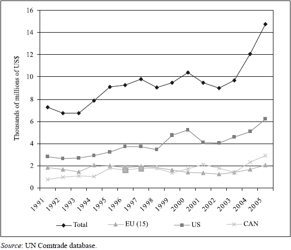
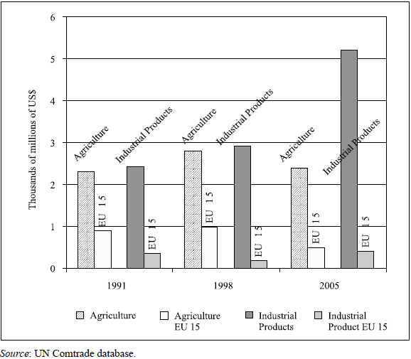
Figure 2 shows the evolution of real Colombian exports in two broad sectors - Agriculture and Industrial Products - and the corresponding exports to the EU (15). The Agricultural sector aggregates the products under SITC code 0, and the Industrial sector aggregates SITC codes 5, 6, 7 and 8. The exports of agricultural and industrial products represented in 2005 85% of total Colombian exports excluding fuels, which are left out because of the influence of volatile world prices on the export of these commodities. It is possible to observe that, while Total Agricultural exports did not suffer significant changes over time, the corresponding value exported to the EU (15) dropped to almost half from 1998 to 2005. As for the Industrial Products, there is a significant increase of exports from 1998 to 2005, both in total terms and to the EU (15) market.

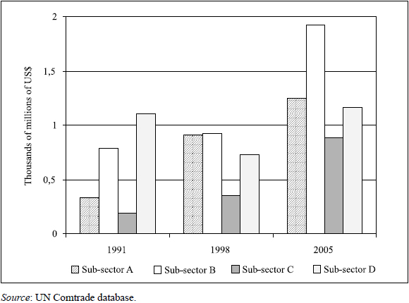
The industrial sub-sectors represented in Figure 3 translate a variety of products. Sub-sector A aggregates chemical products as defined in SITC code 5. Sub-sector B aggregates a diverse range of manufactured products for industrial use defined in SITC code 6. Sub-sector C represents machinery and transport equipment as defined in SITC code 7. Finally, sub-sector D aggregates a diverse range of consumer goods such as apparel, footwear, furniture, etc., as defined in SITC code 8. These four sub-sectors taken together represented 58% of total Colombian exports (excluding fuels) in 2005. During the period under analysis all these sub-sectors registered a progressive increase in the exports. Sub-sector D is the exception: its exports show an irregular behaviour, increasing little from 1991 to 2005.

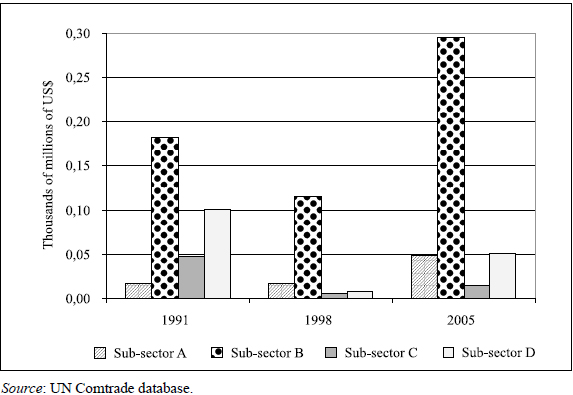
As for Figure 4 it shows the exports to the EU (15) for the same four sub-sectors. Sub-sector A (chemical products) is of low relevance in terms of exports to the EU, but it more than doubled its exports to this economic area from 1998 to 2005. As for sub-sector B, it ranks first in terms of exports to the EU: it decreased its exports from 1991 to 1998, but increased them sharply until 2005. Finally, sub-sectors C and D rank respectively second and third and reduced their exports to the EU during the period under study.

II. Theoretical framework

This section starts by introducing the theoretical foundations of the gravity model. It then presents a survey of the literature involving the gravity equation, exposing some of the most relevant issues related to the discussion about its correct estimation methodology.

A. Theoretical foundations of the gravity model

The gravity equation was first proposed by Newton in 1687 to explain the attractive forces between two objects (Law of Universal Gravitation):

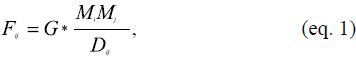
where Fij is the attractive force between i and j, Mi and Mj are the respective masses, Dij is the distance between i and j, and G is a gravitational constant. In 1962 Jan Tinbergen (1969 Nobel Prize Winner) proposed the application of the gravity equation to the study of international trade flows. In this new framework, the general gravity equation applied to trade flows can be expressed as in equation 2:

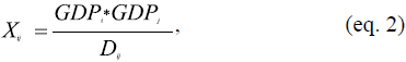
where Fij becomes Xij, the trade flow between i and j, Mi and Mj become the respective economic sizes of the countries involved (GDPi and GDPj), and Dij the distance between countries i and j, which works as a proxy for trading costs. To obtain a linear relationship between these variables, natural logarithms can be applied. The corresponding estimable equation (3) comes as follows:

where the inclusion of an error term captures any other factors affecting the trade flows between the countries. Empirical estimates of showed its value to be positive of magnitude generally in the range 0.7 to 1.2 (Head, 2003: 5). This is easy to understand: when the GDP of the countries involved in a trade relation increases, the trade flow between them is also expected to increase.

In what relates to , its expected sign is negative. When countries are further away from each other they are expected to trade less. In fact, the effect of distance can be interpreted in various ways: as a proxy for transport costs, an indicator of time elapsed during shipment, synchronization costs, transaction costs or cultural distance (Batra, 2004:3).

Equation 3 presents the basic form of the gravity model. Yet, the model generally used is more extensive as it includes additional variables. These variables intend to control or study the effects of other factors thought to influence trade flows (such as the existence of FTAs or borders between trade partners). They generally reflect the existence of some geographical or institutional specificities of the countries involved in trade. In this framework it becomes possible to isolate and explore the effect of a specific factor (or policy) on the trade flows between countries.

Early studies using the gravity model showed good empirical results on explaining trade flows (high R-squared and coefficients' significance). Nevertheless, the gravity model still lacked a theoretical foundation in terms of trade theory. The first to accomplish this was Anderson (1979). He obtained a simple form of the gravity equation from a derivation a Cobb-Douglas expenditure system where he could account for a framework of many goods and transit cost as a function of distance. By considering an economy made of N small and equal countries with a single factor of production Bergstrand (1985) was able to derive a form of the gravity equation from a general equilibrium model of international trade, strengthening this way its theoretical consistency. In a later paper, Bergstrand (1989) incorporated factor endowment differences in the derivation of the gravity equation. He introduced two differentiated product-industries and two factors of productions, showing the gravity model fits both the Heckscher-Ohlin model of inter-industry trade and the Helpman-Krugman models of intra-industry trade.

B. Survey of literature

A large number of authors have used the gravity equation introduced above to explore many features related to trade flows. McCallum (1995) and later Anderson and Wincoop (2003) explored the border effects on the trade flows between Canadian provinces and US states. Both found that Canadian provinces trade impressively more between them than with US states (before NAFTA).

Andrew Rose (2000) made use of the gravity model to study the impact of currency unions on international trade flows. According to his results, "two countries that share the same currency trade three times as much as they would with different currencies" (Rose, 2000). He has also used the gravity equation to estimate the protectionism of the countries (Rose, 2002) by associating the residuals of the model with trade barriers. According to its results Latin America trades less than expected, which is attributed to the existence of higher trade barriers (protectionism).

Rose (2004) used the gravity equation to show whether WTO membership promotes trade. The results reveal no significant evidence that WTO members trade more than non-members. Following these controversial results, Subramanian and Wei (2007) explored whether the asymmetries between trading partners play a role when analysing the WTO as a trade promoting organization. Using an augmented gravity model that takes into account those asymmetries (e.g. developed vs. developing countries, etc.), these authors found that the WTO has actually promoted trade strongly, but this effect was different across country groups and sectors. Countries that participated actively in trade negotiations (industrialized countries) had a larger increase in trade, and the increase in bilateral trade was larger when both trade partners undertook liberalization reforms. The authors also found no significant increase in trade in sectors that did not witness liberalization.

In all these studies the existence of FTAs shows a positive influence on trade. In fact, empirical evidence sustains that free trade agreements increase international trade. Baier and Bergstrand (2007) explored this issue by taking into account the endogeneity problems arising from the use of augmented gravity equations. At stake was the understanding of whether the determinants for the establishment of a FTA were related to the trade flows of the countries involved, which would actually bring about endogeneity problems in the estimation. By applying several techniques they found striking empirical results of a stronger effect of FTAs on trade than that predicted by other techniques.

Some authors have used the gravity model to analyse the impact of trade policies specifically on Colombia. Using a setting similar to that of Rose (2002), Ordenez (2003) quantifies the impact of the commercial policies over the Colombian trade with the world. It shows that Colombia's trade in the second half of the last century was lower than expected (which is attributed to its trade policy). It also defends that Colombia "opened" its economy at a lower rate than the average country. It finally suggests that, in order to correctly estimate the determinants of the Colombian trade, it is necessary to estimate a gravity model specific to Colombia, which is exactly what is done in this paper.

Cárdenas and García (2004) used the framework of Rose (2004) to analyse the trade relations between Colombia and the United States. They found that, taking into account its economic size and geography, Colombian trade level is much lower than expected. Furthermore, in a scenario of a free trade agreement with the US, Colombia would trade around 40% more. At last, withdrawing the US GSP preferences conceded to Colombia (with no free trade agreement) would decrease the trade between these two countries by more than 50%.

While virtually all papers introduced above predict a positive effect of preferential systems on trade, almost none takes into account that different countries are targeted simultaneously with different preferential systems. The study conducted by Persson and Wihelmsson (2006) is probably the one that better analyses these differences. The authors start by constructing a detailed database of the preferences conceded to each of the EU trade partners, classifying the countries according to the preferential system applied to them: the GSP program, the Mediterranean Preferences or the preferences extended to African, Caribbean and Pacific (ACP) countries (this thesis goes even further disaggregating EU's GSP into the consecutive programs applied to Colombia). This database is incorporated in a panel of data covering the period between 1960 and 2002. By using this panel it was possible to estimate the different effects these preferential systems have had on the exports of different groups of developing countries. With the use of an augmented gravity model the authors found that, while other systems of preferences have boosted exports of the privileged countries (ACP and Mediterranean Preferences), the GSP program has provoked no significant increase on their exports. The group of least developed countries, as receptors of additional benefits, was the only one in which this program had significant effects. The authors also found evidence of trade diversion whenever a new country joins the EU (they import less from developing countries when they become EU members). Taking this last point into consideration, the authors suggest that trade preferences have had a positive role on promoting trade, even though other factors had an opposite stronger effect. In other words, the expected positive effect of the GSP has been offset by other factors such as EU enlargements.

C. Correct estimation methodology: the discussion

As stated before, the gravity model generally used includes a number of variables in addition to the basic explanatory variables (GDP and Distance). This way, many authors have included variables to account for geographical, cultural or time-specific characteristics of the countries involved in trade. These characteristics may reflect for example the existence of a border between the trade partners (Border), a common language shared by them (Lang), or the occurrence of a revolution in a specific year (Revolution). These factors can be accounted by introducing a set of dummy variables into equation 4, obtaining this way the following augmented gravity equation:

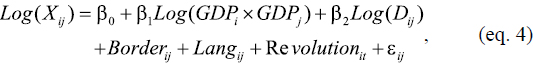
It is possible to think of a variety of other factors that may also influence trade flows between countries and so should be accounted for in the estimation of the gravity equation. Nevertheless, as Anderson and Wincoop (2003) point out, the gravity model estimated as in 3.4 does not correspond to its theoretical background since it omits ‘multilateral [price] resistance terms'. The authors redefined the foundations of the gravity model to take into account for the endogeneity of prices. They applied the model in a theoretical consistent way to the same empirical question as in McCallum (1995): the border effects on the trade flows between the Canadian provinces and the US states. With these new specifications they found that Canadian provinces trade 6 times more among them than with US states (instead of 22 as suggested by McCallum (1995).

Although theoretically consistent, the estimation of the model proposed by Anderson and Wincoop (2003) requires very complex methods (e.g. nonlinear-least-squares). Feenstra (2004: 162) compared this method with the use of simple OLS estimations with the inclusion of country fixed effects. The results obtained under both methods were identical; nevertheless, the latter provides a much simpler set-up for the analysis of trade flows. This way, he suggests that due to its easy implementation, simple Log linear OLS estimation with fixed effects might be a preferred empirical method to obtain average (border) effects on (US-Canadian) trade.

One issue that comes up at this stage is whether to use fixed effects (FE) or random effects (RE) to control for the unobserved factors. The basic difference between these two techniques is that, while FE allows for arbitrary correlation between the variables used (the regressors) and the unobserved factors, RE does not. In the case of time-varying explanatory variables (as in the gravity model), the use of RE is only suitable when a statistical requirement if fulfilled: no correlation between the unobserved factors and the regressors (Wooldridge, 2006: 497). It is thus possible to test which of these two methods (RE and FE) is more appropriate by verifying the fulfilment of this statistical requirement.

In fact, both methods are consistent if the statistical requirements are met. In the case of no correlation between the regressors and the unobserved factors (a statistical requirement for the use of RE), the use of RE is even more efficient. Besides that, RE does not require dropping the variables that are constant over time, something needed with the use of FE. Nevertheless, in the framework of this analysis the requirement of no correlation between the unobserved factors and the regressors is hardly met, which favours the use of FE. Besides that, as Wooldridge (2006: 498) defends, "FE is almost always much more convincing than RE for policy analysis". As this author points out, when using large cannot be treated as random.

If the key explanatory variables to explore are constant over time, it is not possible to use FE. In contrast, if the interest is on time-varying explanatory variables (such as the consecutive European GSP programs), the use of FE is generally the most appropriate. The use FE emerges as the most suitable technique for the analysis at stake. Time and country fixed effects will thus account respectively for all time and country unobserved specific factors that might influence trade flows. As a result, all the variables that reflect time or country specific factors (such as Border, Lang or Revolution) become redundant with the use of this method and must be drop.

III. Empirical framework

This section starts by presenting the specific augmented gravity model to be used in the analysis. The variables used in each of its three versions are here discussed, and the sources of data presented.

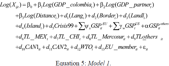
A. The model: methodology and specificities

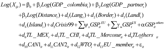
Three different versions of the model will be explored in order to cover a broad range of frameworks used throughout the years. The (panel of) data used covers the exports of Colombia to 167 trade partners between 1991 and 2005. The goal is to understand in which way the consecutive changes to the GSP of the European Union affected Colombian exports. An augmented gravity model is used to explore the effects of these changes.

With respect to the estimations, they are processed in subsequent steps. First, the panel of data is restricted to the countries in which the adjusted export value was higher than US$ 500.000. This follows the methods used by many authors that worked with the gravity model, and intends to eliminate distortions by very small (and not relevant to the analysis) trade partners of Colombia (in the sensitivity analysis this restriction is relaxed). Model 1 is then estimated by OLS. It includes an all range of geographical, cultural, time-specific and institutional control variables as specified bellow.

Model 3 follows the framework suggested by Feenstra (2004: 162) and estimates the model as a Panel of Data with the inclusion of cross-section FE (country-specific), while keeping at the same time the use of year specific FE as in Model 2. In this third version, the inclusion of country FE controls for country specificities constant over time. This way, all cultural and geographical variables (Lang, Border, Landl and Island) become redundant and can be dropped. Furthermore, the use of country FE raises collinearity problems, and so the variables GSPUS1, CAN1 and EU_member must also be dropped.

The explanatory variables used in the three versions of the gravity model are now defined and discussed. Starting with the basic explanatory variables of the gravity model, is the real export value from Colombia (j) to its (i) trade partner in year t. and account for respectively export supply and demand conditions and are expected to have a positive influence on the export level. Following many other authors, these two variables are taken on disaggregated form (instead of the product of and ) to allow for more flexibility in the estimation. is the center-to-center distance (in kilometers) between Bogotá and the capitals or major economics centers of Colombia (i) trading partners. As explained before, this variable is expected to have a negative impact on the export level.

As for the remaining control variables they can be divided in the ones capturing some geographical or cultural characteristics of the trading partners, and the ones capturing the effects of some institutional relations between the countries (such as the existence of a GSP program or a trade liberalization scheme). The dummies and reflect respectively a common language (Spanish) or a common border with Colombia. The first represents cultural and historical ties with Colombia, while the latter captures the often large volume of border trade that neighbouring countries engage in, regardless of their "center-to-center" distance. They are both expected to have a positive coefficient.

The dummies and are related to the fact of having landlocked (no sea cost) or island countries as importers. As these characteristics make it harder for the countries in question to trade (no seaports or no neighbouring countries), their coefficients are expected to be negative. captures the negative shock suffered by the Colombian economy as a result of the 1999 crisis, and so is expected to have a negative impact over the exports.

The set of variables are a comprehensive set of dummies representing the consecutive GSP programs conceded to Colombia by the EU (1-Drug Combat; 2-Progressive preferences according to the sensitivity of the products/no quantitative limitations; 3-further product covered). These binary variables assume the value one if the EU conceded, in year t, a certain x GSP program to Colombia. In general terms, these variables are expected to have a positive impact on the export level, since the GSP program is primarily intended to boost the exports of the recipient country. More specifically, if the consecutive programs applied are more effective or generous in terms of trade concessions, the magnitude of the respective coefficients is expected to be larger.

represents a set of dummy variables representing the consecutive GSP programs conceded to Colombia by the US (1-ATPA; 2-ATPDEA). If these consecutive programs are more effective or generous in terms of trade concessions, the magnitude of the respective (positive) coefficients are expected to be larger.

As the US and the EU are the largest trade partners of Colombia, it becomes relevant to understand the relationship between the two former set of variables. It is possible that in year t both the EU and the US extended the benefits of their GSP programs, and following these changes Colombia increased their exports to US while reducing the exports to the EU. In principal this partly contradicts the expectations introduced above. Nevertheless, it may be the case that, due to the increased attractiveness of the US market (due to further trade concessions), some of the exports to the EU are redirected to the US. If this ‘redirecting effect' (negative) offsets the effect of lower tariffs to the EU (positive), the overall result might be a reduction in the exports to the EU. The opposite is also feasible.

The dummy accounts for the trade preferences conceded by Colombian trade partners (others than the EU and US). , , and represent the tariff reduction schemes agreed between Colombia and respectively Mexico, Chile, Mercosur and other smaller economies. These variables are expected to be positive since a reduction in the tariff level facilitates exports. They are taken disaggregated in order to account for the specificities of the potentially more significant trade partners.

and represent two stages of economic integration with the CAN member countries (Bolivia, Ecuador, Peru and Venezuela): a tariff liberalisation scheme (1) and the constitution of a FTA (2). Both variables are expected to positively influence Colombian exports.

refers to GATT/WTO membership of Colombia's trade partners. The conventional wisdom says that WTO members trade more, and so a positive coefficient for this variable is the most expected. is only relevant for the countries that joined the EU during the time period considered (Sweden, Finland and Austria in 1995; Cyprus, Slovenia, Czech Rep., Estonia, Slovakia, Lithuania, Latvia, Malta, Hungary and Poland in 2004). It assumes the value 1 when these countries become EU members, and tries to capture the presence of a trade diversion phenomenon related to the consecutive EU enlargements (if its coefficient is negative, trade diversion is present). In the absence of this variable, the magnitude of the GSPEU variables could be affected in the sense that it would not only capture the effect of the GSP program, but it would also be affected by possible trade diversion phenomenon.

and represent a comprehensive set of respectively time and country fixed effects. captures variations in Colombian trade flows that are due to trend effects, cyclical fluctuations or crisis such as the one Colombia was subject to in the end of the nineties. captures geographical, cultural or other country specificities not taken into account in previous specifications. For example, for same unknown reason Colombia might trade consistently (over all the years considered) more with country x than country y, despite of their economic and institutional similarity. The inclusion of country fixed effects will take this into account. Finally, is the log-normally distributed error term, which represents other omitted factors influencing the trade flows.

Further specifications are used for the sensitivity analysis. First, the same three version of the model are estimated (i) without restricting the export values as before where only values higher than US$ 500.000 were used. Second, the initial database is restricted in way that it becomes (ii) balanced¹. Third, the data of the 12 (iii) and 15 (iv) old EU member countries is aggregate and taken as a unique importer (Brussels is taken as the center of the EU in the calculation of distance to Colombia; EU12 and EU15 are assumed to be non-Spanish speaking areas). Fourth, the value relative to fuels is subtracted from the total exports, and the model (v) is estimated by using the resultant value (total exports except fuels). This specification is used to eliminate the influence of volatile world prices of these commodities on the exports.

Finally, as a last sensitivity test a time lag between the introduction of the relevant policies (GSPEU and GSPUS) and its translation into the variables that represent them is introduced. This tries to take into account for the possibility that the effectiveness of the policies is anticipated (vi) or retarded (vii). In other words, as there might be some anticipation or friction between policy implementation and the consequent response in terms of trade flows, the inclusion of a time lag might better represent the real effects of the consequent systems in analysis. This is done by changing the timing where the different GSP programs of the EU and the US enter in effect. If anticipation is at place, it would mean that the agents start exporting more/less before the policy is implemented exactly because they expect this change. In the case of the existence of some friction it would mean that the agents would not alter their exporting behaviour exactly after the policy change. This might be the result of bureaucracy (for example the late change of formularies by border authorities) or simple lack of information by the agents.

Regarding the sectoral analysis, the export data is disaggregated and the same estimations are applied to sector export values in order to understand the different developments across the most relevant sectors. First two broad sectors are analysed (agriculture and industry). Secondly, the industrial sector is disaggregated further in four different sub-sectors.

B. Sources of data

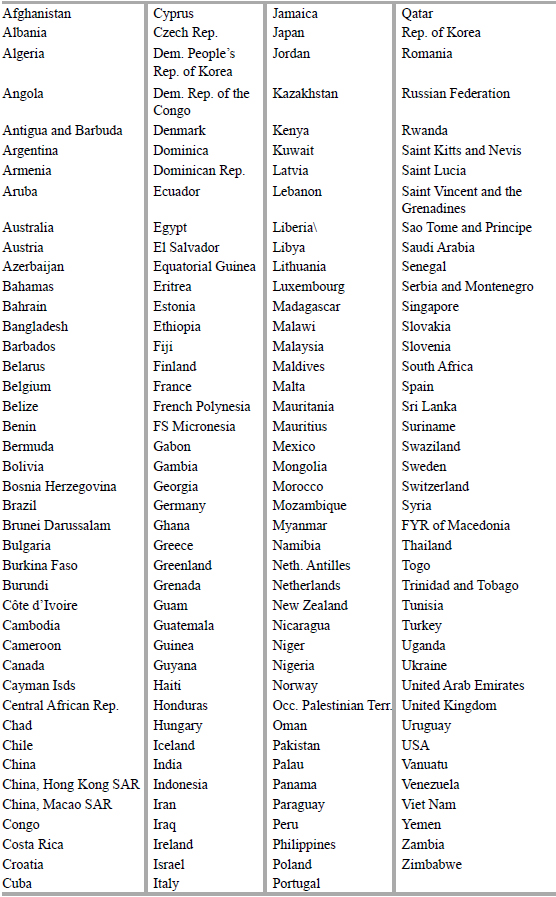
The data used comes from a different range of sources. The export values come from the UN Comtrade database and are denominated in US$ at current prices. It captures the period 1991-2005 for a total of 167 countries (see A3 in the Appendix for the complete list of countries). The export values are deflated by the US CPI, which was obtained from the Bureau of Labour Statistics of the US Department of Labour. The (real) GDP values come from the World Development Indicators (WDI) of the World Bank Database; they are denominated in constant US$ (2000) and are extended to all the years between 1991 and 2005.

The distances between the trading parties were obtained from datasets developed by Haveman and the CEPII. The information for the remaining country specific variables (Language, Landlocked countries and Island) was obtained from the CIA World FactBook.

The information about the different GSP programs was obtained from: the website of the Colombian Ministry of Trade, Industry and Tourism; the UNCTAD website; the WTO Trade Policy Reviews of several countries; the DG Trade website of the European Commission; and the USITC website.

The information on the countries which had some trade liberalization scheme with Colombia (trade liberalization variables) was obtained from the website of the Colombian Ministry of Trade, Industry and Tourism and from the website of the Andean Community of Nations (CAN). The latter was also the source for the information related to the countries that formed a FTA with Colombia. Finally, the dates of the WTO/GATT membership of the respective countries were obtained from the WTO website.

All this information was aggregated in the form of panel of data. The panel is unbalanced in the sense that not all countries have information available for all the years considered.

C. Limitations of the analysis

The models presented above cover a broad range of theoretical frameworks used by many authors that used the gravity equation. Even though, it is crucial to be aware of the limitations of these models.

First of all, it is always possible that some significant variable has been omitted. In this case, the results might be distorted in a way that they lead to wrong conclusions. Nevertheless, in what concerns the institutional variables, they are taken in a much desegregated level in order to avoid this bias. The main trade liberalization schemes (Chile, G3, Mercosur) and the most relevant GSP programs (US, besides the EU) are taken separately so that it is possible to clearly quantify the influence of each of those in the trade flows to be studied. Another set of critics points out that the models characterized as the ones above do not take into account differences in factor endowments among countries (except model 3 – country fixed effects). In other words, countries with different factor endowments will, ceteris paribus, trade more in order to complement each other's lack of specific resources. Melitz (2006: 972) even studied the influence of North-South distance in the trade flows. He found a positive effect of this measure, explaining this exactly with the fact that different latitudes have different factor endowments. However, the use of country fixed effects in model 3 will be able to capture these specific factors, putting aside this criticism.

In what concerns the sectoral analysis, it is still not possible to assess whether the same basic models can correctly be applied to this level of data. Some authors actually applied similar models to analyse trade flows on specific sectors. Even though, different income elasticities of different products might produce unexpected results of some explanatory variables. For example, in theory the influence of GDP_partner might be negative on the exports of inferior goods, which makes sense but goes against the standard predictions of the gravity model. Furthermore, there is a reduced availability of information on exports on a sector level. This way, a small number of observations is used in many specifications of the sectoral analysis, which might influence the quality of the results.

IV. Analysis of the results

This section presents and discusses the results of the estimations performed as specified before. It consecutively examines the results of the analysis of: the aggregated exports, the sensititve tests and the Sectoral Analysis.

A. Results with aggregate exports

Table 1 presents the results of the analysis performed to total Colombian exports following the models presented in the previous section. The importer's GDP (GDP_partner) has a positive and significant effect on Colombian exports in all three models. The fact that this coefficient is statistically lower than 1 implies that, taken into account all other effects considered in the model (specifically the changes in trade agreements), Colombian exports increase less than proportionally with the GDP of its partners. In other words, the model predicts that a 1% increase in the GDP of country A (Colombian trade partner) will result in a less than 1% increase of its imports from Colombia. It may be the case that in a certain period the growth of country A imports from Colombia is higher than its GDP growth, but what the model implies is that GDP growth explains only ~76% (for Model 1 and 2) of the growth in trade, being the remaining related to other drivers such as the changes in trade agreements.

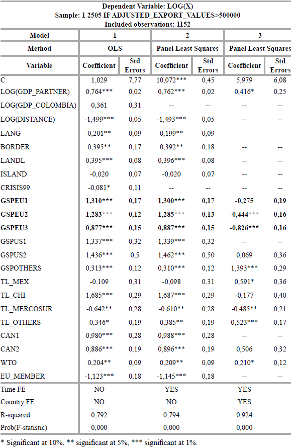
GDP_Colombia (that only entered in Model 1) is insignificant, showing little relevance of this variable on explaining exports. It is nevertheless important to point out that this result is probably due to the fact that there is no variation on the exporting side (Colombia is the only exporter). As for Distance, it is significant, with negative magnitude in both models 1 and 2.

In what relates to the control variables, Lang and Border are significant and have the expected (positive) signs. Landl is also significant but with a positive sign which goes against predictions. Island is not significant. Crisis99 is also not significant, which might seam surprising considering the sharp GDP decline suffered as a result of the 1999 crisis. Nevertheless, the correct interpretation of this result says that, when taking into account the decline in Colombian GDP, it was not observed any higher than expected drop in exports. Besides that, as the results show, Colombian exports are more dependent on its partners' GDP growth than on its own (GDP_Colombia is not significant). This way, it is correct to say that a drop in Colombian GDP will have, as a maximum, a less than proportional effect on exports.

The results for the variables capturing the institutional relations between countries are diverse. TL_MEX is only significant in Model 3, where it presents the expected positive magnitude. TL_CHI is significant with positive magnitude for Models 1 and 2; it is not significant in Model 3. As for TL_Mercosur, it is significant for all models but its coefficients are negative, contradicting predictions. Finally, TL_Others is always significant with positive magnitude, meaning that Colombian exports have been benefiting from trade agreements with other [smaller] economies.

The variables CAN1 and CAN2 are significant for model 1 and 2; they present positive magnitudes (close to one). Theory predicts that the magnitude of CAN2 should be higher than the one CAN1 since the latter represent a higher level of trade barriers between countries. Nevertheless, although the differences are not high, the results show the opposite: the magnitude of CAN1 is slightly higher than the one of CAN2. According to the results for the variable WTO, Colombia trades about 20% more with other WTO members than with non-members (significant for all models).

The variable EU_member is negative and significant in both models 1 and 2. This reveals the existence of trade diversion for the countries that joined the EU during the period in analysis. In other words, when these countries joined the EU, they substituted their imports from Colombia to other EU-members. This was driven by the elimination of trade barriers with the remaining EU member-states. It is then possible to conclude that, in accordance with the results obtained, EU enlargements have a negative impact on Colombian exports. It is interesting to say that, when the variable EU_member is withdrawn, GSPEU3 decreases significantly its magnitude in both models 1 and 2 which means it also captures the existence of a trade diversion phenomenon.

As for the variables representing the US GSP programs, they are significant in Models 1 and 2, where they present positive magnitudes. In thesModels there is a slight increase in the magnitude from GSPUS1 to GSPUS2, which may reveal an increase in the efficiency of the consecutive programs in promoting Colombian exports. In Model 3 the corresponding variable becomes insignificant. GSPOthers is significant and positive meaning that the GSP programs applied to Colombia by other countries (besides the US and the EU) had a significantly positive effect on its exports. The fact that in Model 3 GSPOthers shows a much stronger magnitude is likely due to the use of country FE; this specification takes into account all country-specific effects constant over time, leaving variables such GSPOthers clearly isolated.

The three models revealed high R-squared, a typical characteristic of the gravity model. In simple words, Models 1 and 2 explain around 79% of Colombian exports, while for Model 3 this value reaches 92%. The p-value (Prob(F)) equals approximately zero for the three models, which means that they are overall significant.

B. Discussing the results

At first sight, the results of the previous section do not give a clear answer on whether the European GSP program has been effective on boosting Colombian exports. While Models 1 and 2 predict a positive effect of this program, Model 3 apparently predicts the opposite. This way, the most important question arising at this stage is which Model should be considered more relevant on answering this question.

Even with the use of a variety of (geographical or cultural) control variables, the use of simple OLS as in Model 1 ignores the existence of multilateral price resistance terms. Thus, as noted by Anderson and Wincoop (2003), this specification does not correspond to the theoretical background of the gravity model. The inclusion of both time and country FE will take into account all (time and country) specific factors not considered otherwise. In this framework, and in accordance with what Feenstra (2004: 162) shows, Model 3 is the most theoretically consistent. As a consequence, the results under this Model should be given a stronger emphasis than the ones under the other specifications.

In Model 3 the relative magnitude (increasingly more negative) of the coefficients obtained for the variables GSPEU2 and GSPEU3 give evidence that the consecutive European preference systems have failed to boost Colombian exports during the period under analysis. These results are reinforced by all sensitivity tests performed and presented in the following section. It is nevertheless important to emphasize that the negative coefficients (for the GSPEU variables) in Model 3 should not be interpreted as a negative influence of the European preference system on Colombian exports. As Model 3 includes country FE, it only makes sense to interpret the variables GSPEU in relation to each other²and not in absolute terms (the base level of this effect – common to all three periods –is already taken into account by the country FE). This way, taking into account the use of country FE in Model 3, the relevant conclusion is that the consecutive European GSP programs have been consecutively less efficient on promoting Colombian exports.

In fact, the specifications under Models 1 and 2 also support these conclusions: in all three Models the magnitude of the GSPEU coefficients is consecutively smaller (a result also reinforced in the sensitivity analysis). In other words, the consecutive EU trade preferences conceded to Colombia have been decreasing their effectiveness on boosting its exports over time, a result that clearly goes against predictions. It is definitely remarkable that schemes granting more generous conditions to Colombia are less successful on boosting its exports.

One of the arguments that can be raised to explain the lack of effectiveness of the European GSP is related to the bureaucratic burden often attached to these programs. In order to enjoy the concessions made under such systems the exporters often need to follow complex bureaucratic procedures. By imposing a real cost to these exporters, this complex procedures may constitute a major obstacle to the effectiveness of these programs. On the other hand, the lack of information about such schemes often leads to a low utilization of these export opportunities.

This bureaucratic burden could thus explain the lack of effectiveness of the European GSP program. The changing of procedures (e.g. forms) might even induce an increasing bureaucratic complexity, which would explain the decreasing magnitude of the coefficients. Nevertheless, while there is no strong evidence supporting this argument for the Colombian case, the high utilization ratio of the European GSP program in the Andean region (estimated on 88% in 2003) even contradicts it. Therefore, the bureaucratic burden should not be taken as a factor strongly undermining the effectiveness of EU's GSP program in Colombia.

In order to correctly interpret the results presented in the previous section it is necessary to face the global framework of Colombian trade relations. First of all, it is important to emphasize that in Models 1 and 2 the variables GSPUS present positive coefficients of consecutive larger magnitudes. This means that, while the European GSP program has been decreasing its effectiveness over time, the opposite happened to the corresponding US preference systems. In this framework, it might be the case that concessions made under ATPA and APTDEA (by the US) offset the ones made by the European Union during the same period. If Colombian exporters reacted in accordance, they ‘redirected' the growth of export from the EU to the US.

Nevertheless, in Model 3 the GSPUS variable does not sustain this argument (since it is insignificant). But by analysing the relative growth in exports to the EU and to the US - respectively 13% and 119% in real terms from 1991 until 2005 – it becomes clear that during the period under analysis the US became indeed a much more attractive market to Colombian exports (even if ATPA or APTDEA play no significant role in this change). As a matter of fact the importance of the EU as an export destination has decreased vis-à-vis all other major Colombian trading partners. This is also true when decomposing trade among the major sectors.

Besides that, the variables denoting the FTA to which Colombia belongs within the context of the Andean Community (CAN) also show a positive effect on its exports. As shown in Section I, in 2000 the EU lost its place as the second most important destination of Colombian exports to the CAN. This way, the Andean integration may have also offset the preferences conceded by the EU.

This brings to light a new interpretation of the results. The consecutive European preference systems might indeed be more effective, but at the same time have a low impact on Colombian exports due to the increasing attractiveness of the US market conjugated with a deeper integration of the Andean countries. In other words, favourable US import conditions and the Andean integration process undermined the effectiveness of EU's GSP program. It is thus reasonable to say that without the consecutive changes in the European GSP system Colombian exports to the EU would have been even lower than they actually were.

Another interesting feature is related to the impact of EU enlargements in the European imports from Colombia. The variable EU_member presents a significant coefficient of highly negative magnitude. This means that, whenever new members join the EU, their imports from Colombia decrease. This is a typical trade diversion phenomenon, which is also consistent with results achieved by to Persson and Wihelmsson (2006). The two EU enlargements that happened during the period under analysis might partially explain the decreasing effectiveness of EU's GSP. For instance the 1995 EU enlargement coincided with the introduction of further trade concessions to Colombia (GSPEU2). As an example, before joining the EU Sweden applied no tariffs to its imports. After joining the EU, its imports from non-EU members became subject to the common European tariff regime, a situation which provoked a reduction in its imports from Colombia. European imports from Colombia were thus affected on a negative way by this trade diversion phenomenon. Once again, if the EU would have not expanded its trade concessions to Colombia, it is likely that Colombian exports would have been even lower than the levels actually registered.

Even though the lack of effectiveness of the European GSP program might be explained by factors exogenous to the program itself (increase in the attractiveness of the US market, CAN economic integration and EU enlargements), the fact is that in the period under analysis it failed to boost Colombian exports. Taking this into account, the establishment of an FTA with Colombia would probably be a more effective way of promoting its exports.

The scenario of a FTA between Colombia and the EU would bring more predictability and less uncertainty to Colombian exporters, working as a stimulus for the establishment of long-term trade relationships between both economies. Furthermore, the establishment of a FTA with the EU would eliminate the bureaucratic burden as a factor that possibly (although unlikely) hinders Colombian exports.

C. Sensitivity analysis

As can be observed in Table 2, a total of seven sensitivity tests were applied to the analysis of total Colombian exports. Here the emphasis will be put on the sign and magnitude of the objective variables: GSPEU. Test (i) and (ii) show similar results to those of the main analysis. In both Models 1 and 2 the difference in magnitudes of the variables GSPEU is larger: GSPEU1 is higher and GSPEU3 is lower than before. As for Model 3, the significant variables are also negative, and in specification (ii) their magnitude is stronger (more negative). In Tests (iii) and (iv) all the coefficients become insignificant. By aggregating the EU countries in a single yearly observation there is a clear loss of information, which turn out to be evident in the results. Test (v) shows a decrease in the magnitude of the GSPEU variables for Models 1 and 2. As for Model 3, the results for specification (v) are all significant and, as before, of increasingly negative magnitude.

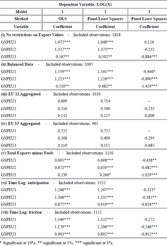
The results presented in specifications (vi) and (vii) take into account the possibility of respectively anticipation and friction in the agent's responses to policy implementation. When compared to the initial estimation results presented on Table 5.1.1, these specifications show no significant changes, whether on significance or magnitude of the objective variables. This way, it is not possible to identify neither anticipation nor friction effects on this policy changes. Nevertheless, the most relevant conclusion for this study is that the relative magnitudes of the objective variables do not change, which certainly gives more robustness to the results achieved before.

An additional interesting result concerns the variables GSPothers and TL_others. In all specifications they are significant and positive (the exception is GSPothers, which is insignificant in Model 3 of sensitivity test (v)).This means that the trade concessions Colombia enjoys under these schemes have been clearly effective. Nevertheless, taking into account the reduced importance of these countries in terms of Colombian exports, such trade concessions are overall less relevant to Colombia.

D. Sectoral analysis

The analysis on the disaggregated exports revealed different results across sectors (see table 3). Staring with agricultural products, although Models 1 and 2 shows evidence of a positive effect, Model 3 presents highly insignificant results, introducing some uncertainty over the real effect of EU's GSP over this sector's exports. It is important to say that the 2002 GSP revision (GSPEU3) suspended all duties applicable to those products. It would thus be expected a relatively stronger positive magnitude for GSPEU3 as actually Model 2 shows. Nevertheless, taking all results obtained it is not possible to conclude with confidence whether EU's GSP program had a positive effect or no effect at all over Colombian agricultural exports.

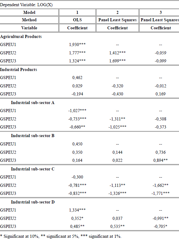
As for the Industrial Products, the results are insignificant for all three models. As the sector defined as Industrial Products is composed of a wide range of different goods, these results might be the outcome of a different effectiveness of EU's GSP on promoting exports in different groups of goods.

Industrial sub-sector A shows negative coefficients in Models 1 and 2, and insignificant ones in Model 3. It is thus possible to say that the changes on EU's GSP did not contribute to boost Colombian exports of ‘Chemicals and related products' (A).

Industrial sub-sector B, which is formed by manufactured goods mainly for industrial use (leather, iron, steal, etc.), only registered significant coefficients in Model 3. According to these results GSPEU3 had a positive effect over Colombian exports of these products. In fact, from 1998 to 2005 the share of exports to the EU (15) of these products raised from 12% to 15%, showing an increase in the relevance of the EU market for this category of goods. Besides that, it is important to say that this category of products is the largest both in terms of total Colombian exports of industrial products (37% of total industrial exports in 2005) and in terms of industrial exports to the EU (72% of industrial exports to the EU in 2005). This way, the results suggest that the further concessions made by the EU in terms of the product coverage in 2002 provided a true advantages to Colombian industry.

As for sub-sector C (machinery and transport equipment), the results give strong evidence that the European preference system failed to facilitate its exports. It is nevertheless relevant to point that this sub-sector is the smallest in terms of exports among the ones analysed, and so its underperformance does not represent a significant difficulty in terms of overall Colombian exports.

Finally, sub-sector D presents contradicting results. While Models 1 and 2 show a positive influence of the European GSP on its exports, Model 3 gives evidence of the opposite. Even though it should be given a stronger emphasis to the results under Model 3 (for theoretical consistency reasons explained in the previous section), it is possible to present arguments in both ways.

On the one hand, the recent (global) trade liberalization in the context of the Agreement on Textiles and Clothing³ (ACT) has been progressively removing the barriers to the trade of goods under this category (D). This would explain the higher than average exports of these products (positive coefficients under Models 1 and 2). Nonetheless, it would at the same time eliminate the efficiency of the European GSP as the reason for these higher exports. On the other hand, and partially as a result of the progressive liberalization under ATC, China and other Asian countries have in recent years been expanding their exports of the manufactured goods under category D to the EU. This way, the framework of more intensive competition would explain the lower than average exports in sub-sector D. Overall, for one reason on another, the European GSP program most likely failed to boost exports in sub-sector (D).

Overall, only for sub-sector B it is possible to find a positive effect of the European GDP in Model 3. Sub-sector D presents positive coefficients in Models 1 and 2 but those results are not supported by Model 3, which presents negative coefficients. As for the remaining (A and C), the results are always negative or insignificant.

V. Conclusion

This study made use of a gravity model specific to Colombian exports to analyse the effectiveness of the European generalized system of preferences on boosting them. By taking Colombian trade patterns as the basis of the analysis this approach made possible the estimation of the specific determinants of its trade flows. Moreover, by disaggregating the European GSP systems in accordance to the progressive changes introduced during the period under analysis it became possible to analyse the effectiveness of this policy in dynamic terms.

The results achieved present evidence that the European Generalized System of Preferences had little success on promoting Colombian exports to the EU. Most importantly, it shows that during the period under analysis this program revealed a progressive lower effectiveness. These results must nevertheless be interpreted under the context of an increasingly more efficient US preference system, a deepening of the Andean integration, and the occurrence of EU enlargements during the period under analysis. All these factors contributed to a reduction of Colombian exports to the EU market that is not attributable to the lack of efficiency of the European GSP. In this framework, it might be the case that EU's GSP actually had a positive effect, but these other factors had a negative and larger effect over Colombian exports to the EU market.

On a sectoral level the largest category of industrial goods in terms of Colombian exports (sub-sector B - manufactured products mainly for industrial use) shows evidence of a positive effect of the European GSP program on its exports. The results suggest that the further product coverage conceded to Colombia in 2002 on the framework of the European GSP did make a difference in terms of its exports of this category of goods. In fact, the share of exports to the EU of this group of goods grew from 12% to 15% between 1998 and 2005. As for the remaining sectors, the results are either insignificant or conflicting. Evidence points to the failure of EU's GSP on promoting exports in sub-sectors A, C and D.

In terms of future research on this topic it would be relevant to extend the set-up used on this study to all CAN member countries. Without loosing the specificity of the model for this region it would then be possible to analyse the effectiveness of the European preference system on this group of countries. Besides that, in a context where the share of Colombian goods exported to the EU has been decreasing, it would be very important to compare the role played by the EU with the one played by the US in what concerns to trade with this region. As for the sectoral analysis, it would be very interesting to match its results with firm/product level data in order to understand which firms or products benefit the most/less from the concessions made under the European preference system.

Appendix

Table A1. Colombian trade relations.

A2. The three version of the Model

Equation A1. Model 1, estimated by OLS.

Equation A2. Model 2, Time Fixed-Effects.

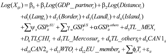
Equation A3. Model 3, Time and Country Fixed-Effects.

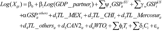
where t denotes the year, j denotes Colombia, i its trade partners and x and w denote the different GSP program conceded to Colombia respectively by the EU and the US.

A3. List of Countries in the Database

FOOT NOTES

1. The term ‘Balanced' is used in the sense that all information is available for considered countries in all relevant year.

2. In Model 3 the coefficient for GSPEU1 is not statistically different from zero; the coefficients for GSPEU are consecutively smaller GSPEU3 < GSPEU2 < GSPEU1 = 0 = base level.

3. The Agreement on Textiles and Clothing introduced a phasing-out scheme for the import quotas applied to the Textile and Clothing sectors. It was broke up into four liberalization stages (1995, 1998, 2002 and 2005) in which the existent quotas were progressively eliminated.

References

1. Anderson, J. E. "A theoretical foundation for the gravity model", American Economic Review, 69(1), (1979): 1006-116.        [ Links ]

2. Anderson, J. E. and van Wincoop, E. "Gratity with gravitas: A solution to the border puzzle", American Economic Review, 93(1), (2003):170-192.        [ Links ]

3. Baier, S. L. and Bergstrand, J. H. "Do free trade actually increases member's international trade?", Journal of International Economics, 71(1)(03), (2007):72-95.        [ Links ]

4. Batra, A. "India's global trade potential: The gravity model approach", Indian Council for Research on International Economic Relations, Working Paper, 151, (2004).        [ Links ]

5. Bergstrand, J. H. "the gravity equation in international trade: Some microeconomic foundations and empirical evidence", The Review of Economics and Statistics, 67(3), (1985):474-481.        [ Links ]

6. Bergstrand, J. H. "the generalized gravity equation, monopolistic competition, and the factor-propotions theory in international trade", The Review of Economics and Statistics, 71(1), (1989):143-153.        [ Links ]

7. Cárdenas, M. y García, C. "El modelo gravitacional y el TLC entre Colombia y Estados Unidos", Fedesarrollo, Working Paper Series, 27, (2004).        [ Links ]

8. European Commission. "The European Union's generalized system of preferences", Directorate General for Trade, 4, (2004).        [ Links ]

9. European Commission. "Global Europe competing in the world: a contribution to the EU's growth and jobs strategy", External Trade, 10-11, (2006).        [ Links ]

10. Feenstra, R. Advanced international trade: Theory and evidence. Princeton University Press, (2004).        [ Links ]

11. Head, K. Gravity for beginners. University of British Columbia, Faculty of Commerce, (2003).        [ Links ]

12. McCallum, J. "National borders matter: Canada-U.S. regional trade patterns", The American Economic Reviews, 85(3), (1995):615-623.        [ Links ]

13. Melitz, J. "North, South and distance in the gravity model", European Economic Review, 51(2007), (2006):971-991.        [ Links ]

14. Ocampo, J. R. ¿ No TLC? El impacto del Tratado en la economía colombiana. Bogotá, Grupo Editorial Norma, (2007).        [ Links ]

15. Ordenez, X. C. Impacto de la política comercial en Colombia, (2003).        [ Links ]

16. Persson, M. and Wihelmsson, F. Assessing the effects of EU trade preferences for developing countries. Lung University, Department of Economis, (2006).        [ Links ]

17. Rose, A. "One money, one market: Estimating the effect of common currencies on trade", Economics Policy, 30, (2000):7-45.        [ Links ]

18. Rose, A. Estimating protectionism through residuals from the gravity model. International Monetary Fund, Background for Chapter III of the September 2002 World Economic Outlook, (2002).        [ Links ]

19. Rose, A. "Do we really know that the WTO increases Trade?", American Economic Review, 94(1), (2004):98-114.        [ Links ]

20. Subramanian, A. and Wei, S.-J. "The WTO promotes trade, strongly but unevenly", Journal of International Economics, 72, (2007):151-175.        [ Links ]

21. Trade Policy Review Body. "WTO trade policy review–Colombia", document WT/TPR/172, (2006)        [ Links ]

22. Wooldridge, J. M. Introductory econometrics–A modern approach (3 rd Ed.). Michigan State University, (2006).        [ Links ]