Imagining Education: Educational Policy and the Labor Earnings Distribution

Educación imaginada: política educativa y la distribución de ingresos laborales

Diego Amador*

* University of Pennsylvania. 160 McNeil Building, 3718 Locust Walk. Philadelphia, Pennsylvania 19104-6297. amadord@sas.upenn.edu. I would like to specially thank Raquel Bernal for all of her advise, ideas and support; and to Ximena Peña for her comments, uninterested help and encouragement. I'm grateful to Juan Camilo Cárdenas, José Leibovich and two anonymous referees for their suggestions and to the three Ms and E for their unconditional support.

Abstract

This paper simulates, within a partial equilibrium framework, the scenarios resulting from the implementation of several educational policies. Then, policies are compared according to their hypothetical results in terms of labor earnings inequality, as measured by the Gini coefficient. Results suggest that educational policies which attempt to guarantee medium qualification produce the lowest inequality even if dispersion in schooling years is high. Policies which attempt to raise tertiary education coverage but do not raise high school coverage as well, lead to rising inequality.

Key words: Educational policy, economic inequality, schooling. jel classification: 128, J24, J38.

This article was received January 29, 2009, modified September 21, 2009 and finally accepted February 19, 2010.

Resumen

En este trabajo se simulan, dentro de un marco de equilibrio parcial, los escenarios que resultarían de la implementación de una serie de políticas educativas. Dichas políticas son comparadas a partir de sus efectos hipotéticos sobre la desigualdad en los ingresos laborales, medidos a partir del coeficiente de Gini. Los resultados indican que las políticas educativas que garantizan la educación media universal producen la menor desigualdad. Y aquellas políticas educativas que aumentan la cobertura en educación terciaria sin garantizar primero un nivel medio llevan a una mayor desigualdad.

Palabras clave: política educativa, desigualdad económica, escolaridad.

Clasificación jel : I28, J24, J38.

Introduction

Educational policy affects the schooling years of individuals in a given society. Thus, it potentially has an effect on the distribution of labor earnings throughout the population. Nevertheless, economic literature does not provide policy makers with means to predict these effects. This paper compares the results of a series of empirical exercises in which the scenarios, in terms of labor earnings inequality, that would emerge after the implementation of a set of plausible educational policies are predicted. All of the above is developed within a partial equilibrium framework, in which only labor earnings are affected by the educational policies.

In order to simulate the effects of the different educational policies on the distribution of earnings, a methodology that has been widely used in decompositions of changes in earnings inequality (Bourgignon and Ferreira, 2005) is applied. The educational policies are represented by the objective distribution of schooling years across the population associated with each one of them. The main advantage of this methodology is that it allows identifying and isolating the effect of each distribution of schooling years on the distribution of earnings, conditional on the

distribution of other individual characteristics correlated with earnings and the prices of those characteristics. The estimated prices for 2004 are used.

Several conclusions arise from the described exercises. First, guaranteeing medium qualification (high school) appears to be a powerful and necessary way of achieving lower inequality. Educational policies which attempt to raise average schooling years or tertiary educational coverage but do not start with full high school coverage are not efficient at lowering labor earnings inequality. Also, composition of the schooling distribution, and not only its variance, proves to be of great importance when relating it to the labor earnings distribution. Thus, the results suggest the possibility of achieving scenarios in which a high variability in schooling years coexists with low earnings inequality. In particular, an ambitious schooling distribution¹ in which high school is guaranteed and half of the labor force has a college education, generates good results in terms of earnings inequality without making sacrifices in terms of earnings level, at the same time that it is has a relatively high dispersion of schooling years. Finally, since some of the educational policies included are nested within other of these policies, a very general analysis can be made about two different paths towards a schooling distribution with a higher proportion of high skilled labor.

I. Labor earnings inequality and the educational expansion

Figure 1 shows the evolution of labor earnings inequality, measured by the Gini coefficient, during the period 1980-2003 in Colombia. Just as it has been widely documented by economic literature, inequality rose systematically since the end of the 1980's. At the same time, average years of schooling went from about 6.5 in 1982 to slightly above 8 in 2000 (figure 2). During this same period, the standard deviation increased as well. The coefficient of variation fell to about 0.52, though (almost 0.05 less than it was ten years before). Nevertheless, these changes cannot fully acknowledge relevant variations in the composition of the schooling distribution. As figure 3 shows, the outstanding growth in the proportion of people with high school or more was mainly driven by the increase in the percentage of the population who completed high school but has no tertiary education, and complemented, although not so strongly, by those with some tertiary education and the decrease of the relative size of those with no schooling.

Thus, one could expect that the particular composition of the schooling distribution would affect the earnings distribution. In other words, it is definitively important to take into account the exact way in which schooling is distributed, and not only the variance of this distribution, in order to understand the relationship between education and economic inequality. Clearly, the observed changes in the Gini coefficient ought not to be explained only by the changes in the schooling distribution. Nevertheless, a great deal of the variation in labor earnings seems to be determined by the dispersion in the schooling of individuals. Cárdenas and Bernal (1999) have shown that, in 1996, 36% of the earnings inequality could be explained by schooling alone². Furthermore, in a hypothetical scenario in which all individuals had identical observed characteristics and, therefore, the variance in their labor earnings was solely due to unobserved characteristics and stochastic shocks, the estimated Gini coefficient would be 0.173. If schooling was allowed to vary too, the Gini coefficient would climb to 0.346, accounting for approximately 35% of observed inequality. Compared to this, potential experience (the other individual characteristic measuring human capital accumulation) would account for just 10% of inequality.

Thus, understanding the connection that has been discussed becomes fundamental for the analysis of the determinants of the behavior of earnings inequality during the last decades, as well as in the attempt of designing equality enhancing public policies. The former has been developed through different empirical strategies (Cárdenas and Bernal, 1999; Núñez and Sánchez, 1998b; Santa María, 2004; Vélez, Leibovich, Kugler, Bouillon and Núñez, 2005). This work intends to contribute in the latter.

II. Labor earnings distribution, educational policy, and the schooling distribution

Educational policy can be a very ambiguous term and, so far, it has been used in this paper without giving any clear and precise definition. Even though educational policy includes a great variety of actions, goals, perspectives, etc., it will be used here to refer, exclusively, to the precise goals in terms of enrollment in the different schooling levels and the means for achieving those goals. Therefore, it will make no reference to any other dimensions of educational policy, such as quality, ideology, curriculum, or any other element that may be included in a broader definition. Thus, it is a conceptual and terminological simplification. Within this particular and narrowed dimension of educational policy, it is reasonable to think about the goals of policy makers in terms of an objective schooling distribution within the relevant age range. For example, when someone talks about universal coverage in basic education (Colombian 9^th grade), she might be thinking about a schooling distribution in which all of the individuals have, at least, 9 years of schooling. Based on the above, one of the main assumptions supporting the work developed in this paper is that different educational policies can be represented by their corresponding objective schooling distribution, which is, according to what has been stated, a plausible assumption.

Thus, the basic concern underlying this paper is that of the relationship between schooling and labor earnings distributions, understanding the former as the plausible representation of the goals of given educational policies. In particular, it is worth asking oneself about what kind of schooling distributions would be associated with less unequal earnings distributions. If there exists at least a partial answer to this question, a connection between the schooling distributions and the particular

educational policies they attempt to represent could be posed. Based on this connection, useful criteria for educational policy design could be created, in terms of its effect on labor earnings inequality.

III. Data

All of the estimations in this paper are based on the Encuesta Nacional de Hogares and the Encuesta Continua de Hogares (Household survey)³ for the stages corresponding to the third quarter of 1985, 1995 and 2004. Information on individual years of schooling (used also

for the construction of level premia); age (used in the construction of potential experience⁴); occupation (construction workers, employees, domestic service employees, self employed, business owners and other earners); metropolitan area of residence (Bogotá, Barranquilla, Bucaramanga, Medellín, Manizales, Cali and Pasto); marital status (cohabiting, married, widowed, single, separated/divorced); household size (in terms of household members and household members under 10); relationship with the head of household; and individual labor earnings is used.

The sample has been restricted based on several criteria. First, only data from people living in the 7 largest cities is included. This is done to assure comparability between samples for the different stages of the survey. People reporting more than 84 hours worked during the previous week are excluded⁵ too, in order to reduce probable measurement error. Finally, with that same purpose, observations in the top and bottom 1% of the labor earnings distribution are excluded as well. As a result of all of the above, the sample size for the estimation of the earnings functions is 47,179, where 23,199 of those observations are reported earners (2004 sample)⁶.

IV. Literature review: A selection

The following literature review is focused on three subjects: work attempting to explain the rise in inequality during the 1980's and 1990's in countries other than Colombia (mainly usa); in Colombia; and research that includes some prediction of the effects of educational policy. This kind of literature is, to say the least, abundant. Thus, this review is not intended to be exhaustive. Quite the opposite, the idea is to set some relevant examples, as well as to introduce fundamental conclusions of some seminal papers.

The observed rise in inequality during the 1980's and 1990's triggered, in many countries, a proliferation of economic literature which tried to explain the determinants of such a change in the trend. For example, Juhn, Murphy and Pierce (1993) found that a great deal of this phenomenon could be explained by changes in the unobserved components (attributed to unobserved ability) of wages, and by the different timing of these and the changes in observables. The American rise in inequality of the 1980's would be owed to an increase in the wages of high skilled workers (returns to observed ability), as well as an increase in the returns to unobserved ability.

Katz and Murphy (1992) argued that, besides the growing demand for skilled workers, unobserved ability and female labor, one of the main determinants of the changes in the American wage structure between 1963 and 1987 was the dynamics in the relative supply of skilled labor. DiNardo, Fortin and Lemieux (1996) added institutional and normative components to the explanation (i.e. changes in the union structure) and proposed the behavior of the minimum wage as another basic determinant. Mincer (1996) found that the within educational group inequality was the largest contributor to overall inequality, once other variables are controlled for. Following Juhn etal. (1993), he identifies these changes with rising returns to unobserved ability, which would be due to technological dynamics.

Murphy, Riddell and Romer (1998) analyze the changes in earnings inequality in the United States and Canada, and attempt to relate them with technological change. They find that the behavior of inequality can be explained by changes in relative supply of skilled labor and changes in technology which raise the demand for unobserved ability. According to them, the rise in inequality would have been stronger in the Canadian case if there had not been a progressive equalization in the supply of differently skilled kinds of labor. Beaudry and Green (2000) try to explain the Canadian case with a totally different set of arguments, based on the hypothesis of a systematic deterioration of labor market conditions. They conclude that younger cohorts face a lower earnings profile than older ones throughout their entire lifetime.

Finally, Johnson (1997) finds that the relative demand for skilled worked has followed a rising trend since the 1940's, which experienced an important acceleration starting at the beginning of the 1980's. The same did not happen with the relative supply, which lagged during this last period. From this point of view, the rise in earnings inequality comes from these different dynamics in relative supply and demand. Although several explanations could be posed, the rise in unobserved ability due to technological change seems to be the most reasonable to the author.

Colombia was not an exception to the rising inequality trend (as it was shown in figure 1) and a vast economic literature has been produced on the subject. Núñez and Sánchez have exhaustively documented changes in the Colombian wage structure (1998a), the determinants of changes in labor earnings inequality (1998b) and the changes in the decisions of Colombian households (2002) during the 1990's. Generally speaking, they find robust and consistent evidence of the importance of education in all of these processes, especially through the observed changes in relative prices and supply. According to them (1998b), schooling alone can explain 20% to 30% of the variation in inequality. They observe differential dynamics between male and female labor prices too. Besides that, within sector mobility and the deterioration of overall labor market conditions are found to be powerful and fundamental components of the observed changes in inequality.

According to Santa María (2004), the recent Colombian labor market conditions can be characterized by decreasing returns to intermediate skilled workers and increasing relative wages of women and skilled workers. He rejects the hypothesis of a relationship of these and the structural reforms that took place in Colombia at the beginning of the 1990's (openness and trade liberalization). The explanation could be found, he concludes, in the variations of the skill composition of the labor force and skilled bias technological change.

Vélez et al. (2005) make a decomposition of the observed changes in inequality, based on the same methodology used later on this paper (Bourguignon and Ferreira, 2005). Based on their estimations, they classify determinants as persistent and fluctuating forces. The first group includes, on the one hand, socio-demographic conditions such as the schooling distribution, which are the result of long term trends. The fluctuating determinants include, on the other hand, some of the most important determinants (i.e. the rising returns to skill) which, nonetheless, obey to transitory conditions. Generally speaking, their results agree with what had been found by Núñez and Sánchez (1998a, 1998b, 2002). But besides all of these, and contrary to their expectations, they find that the equalization of educational endowments led to a deterioration of the income distribution in urban areas (Vélez et al, 2005, p. 127).

Taking a different methodological perspective, in recent years, technological innovation has allowed the full estimation of structural models in diverse fields including labor economics. These estimations include, in many cases, the simulation of the effects of particular public policies in a specific framework. There is no intention here to survey this literature. On the contrary, just a couple of examples of public policy simulations are set. They are completely different in nature to the ones developed later on, though.

Keane and Wolpin (1997) estimate a model of schooling, labor force participation and occupational choices. Based on it, they evaluate, for example, the consequences of introducing college subsidies. Keane and Wolpin (2001) ask themselves about the effects of liquidity constraints and parental transfers on the decisions of human capital investments and labor market choices. They simulate scenarios which include subsidies, relaxing the constraints and equalizing parental transfers. They find, among other things, that liquidity constrains are not as important as parental transfers in the determination of the decisions mentioned above. Both of these works, as most of the literature does, evaluate only partial equilibrium effects of the public policies.

Opposite to this literature, this paper develops some empirical exercises based on reduced form models instead of structural models. The data available in Colombia does not allow doing something of that type. Despite this restriction, the greatest advantage of the methodology used here is that it allows the evaluation, in a rigorous manner, of the partial equilibrium effects and consequences of educational policies which cannot be observed in historical data, isolating the effects of the particular variable of interest.

V. Methodology

A. Baseline methodology

The methodology proposed by Bourguignon and Ferreira (2005) is basically one designed for decompositions of changes in earnings distributions between two periods. The first step⁷ is to estimate a conditional earnings function for different moments in time. The assumption here is that individual earnings are correlated with other observed characteristics such as schooling, experience, gender, marital status, etc.; the market prices of those characteristics; and an error term including unobserved characteristics and stochastic shocks. Thus, the following can be written:

where {y_i}^t are the observed labor earnings in time t, and χ_i, Θ_t, Π_t are the distribution of the observed characteristics, the prices of those characteristics and the distribution of the error term in time t. In the particular case of individual labor earnings, the distributio D(χ_t, Π_t,Θ_t) can be easily estimated through a Mincer equation, which can be expressed this way:

Accordingly, the function generating distribution D( ) would be:

The next step is to define the counterfactuals in the way Bourguignon and Ferreira do. The changes needed in order to simulate the effects of educational policies will be shown later.

Knowing X for two given moments in time t and s, F( ) can be estimated for these two cross sections. In this paper, this estimation includes the correction of selection bias by using the Heckman mle process. Consequently, there will be

The counterfactuals are obtained by simply simulating the earnings distribution after substituting the elements of F( ) from t to s or vice versa. For example, the counterfactual

could be created, in which an earnings distribution is simulated using the observed characteristics in t, the estimated distribution of residuals for that same period, but the prices of s. This counterfactual can be interpreted as the earnings that individuals with the characteristics of t would have had if the prices would have been those of s. Since what it is generated through the simulation process is a distribution, inequality measures can be estimated on the counterfactual.

A possible extension of this process is to do these exercises with hypothetical X distributions which do not necessarily come from observed data. This procedure is different form the one proposed by Bourguignon and Ferreira because it does not intend to decompose changes in the distribution into changes in the elements of F ( ). Nevertheless, this methodological variation allows the prediction of the consequences of educational policies which can be represented through those hypothetical X distributions, even if these policies cannot be observed or proxied through actually observed data.

B. Educational policy counterfactuals

According to what was mentioned in the previous section, a counter-factual in which the distribution of X is created arbitrarily could be thought of. Specifically, artificial variations could be generated on the data included in X_t (the observed distribution of X in t). Since X_t is really a matrix in which each column is a particular variable or characteristic, the arbitrary Xs would leave all of those columns (variables) unaltered except the one containing the data on schooling (thus its distribution). Schooling data is changed in order to represent a specific educational policy. In this way, the counterfactual

Is obtained, where χ_c is the counterfactual distribution of X (only different from X_t in the schooling data), is the estimated distribution of the random term estimated in t, and are the parameters estimated in that same year.

Therefore, the comparative analysis is established on the different counterfactual distributions of labor earnings {y_i}^c→t which come from the different χ_c distributions (the schooling distributions included in them) and their interaction with parameters :

The comparison between two distributions {y_i}^c→t and {y_i}^h→t is based on any inequality measure (Gini coefficient or Theil's entropy measure, for example), which allows the distributions, and their corresponding educational policies, to be ranked according to the level of inequality they produce, taking the distribution of other characteristics, the estimated prices and the distribution of the error term as given. Formally, an earnings distribution c will be considered to be better than another distribution h in terms of inequality if

I [] could be any inequality measure. In this paper, it will be the Gini coefficient, although Theil's entropy measure is also reported in the results.

Since the only thing that makes {y_i}^c→t different from {y_i}^h→t is the schooling distribution in the generating process (other observed characteristics are identical, as well as the residuals), the above allows to conclude that if c is better than h, then X_c is better than X_h. This really means that schooling in X_c is better than X_h. Under the assumption that schooling in c and h are the representations of educational policies c and h, educational policy c is said to be better than policy h.

Finally, it is worth noting that any effect of the educational policies on the labor income distribution is conditioned on the other observed characteristics and their prices. About the former, the ones observed in 2004, which are the most recent ones available, are used. About the latter, the results are robust to the year in which they are estimated.

C. Earnings and participation functions

As it was mentioned on the previous section, the distribution of earnings, conditional on other characteristics can be easily estimated through a Mincer equation. Off course, there are other more sophisticated ways of estimating some of the elements included in a Mincer equation. Heckman, Lochner and Todd (2006) have shown that the coefficients of schooling in this type of models cannot be interpreted as the internal return rate to schooling. Nevertheless, there is no interest here in estimating such thing. Human capital investments of individuals are not being modeled. Quite the opposite, the distribution of schooling is taken as exogenous, since it is the representation of some particular objectives in a given educational policy. Thus, the Mincer equation is just used as the conditional distribution of log labor earnings or, as it is stated by Peracchi (2006), the statistical function of labor earnings.

According to this, the particular specification of the Mincer equation is:

which includes the individual's schooling years, potential experience (in linear and quadratic forms), high school and college premia, and city, occupation and marital status fixed effects.

The choice of the particular form for schooling in this equation (linear term plus two level premia) is owed to the assumption of discrete changes in earnings at these specific points of the schooling distribution. It is a standard specification in economic literature and a widely used one in Colombia (i.e. Núñez and Sánchez 1998a y 1998b).

This estimation has to be corrected for possible selection bias. This process is done through the Heckman method, where the Mincer equation is jointly estimated with the selection equation, in which the probability of participating is determined as follows:

where female_householdhead is 1 if the household head for the individual's household is a woman and 0 otherwise; householdhead is 1 if the individual is the head of his household and 0 otherwise; hhincome_spouse and hhincome_parent are the head of household's income in case he/she is the spouse or the parent of the individual, respectively.

Since this selection equation is, in fact, a raw modeling of the decision of participating in the labor market, the effects of educational policies on it could be taken into account too. However, this would require assuming that all of the possible rises in participation rates due to higher overall schooling can be absorbed perfectly by the labor market. No need to be said, this is a very strong assumption and an unlikely thing to happen. As it is shown in table 1, the difference in predicted occupation rates between some of the policies would be of more than 20 percentage points in some cases. This rules out this option almost automatically. Thus, baseline results are based on another assumption which is just as strong but less unlikely than this one. Participation decisions are assumed to remain unaltered by educational policies.

Off course, the real scenario must be somewhere in between these two situations. Fortunately, relative results are identical when participation effects are and are not included in the simulations. Nevertheless, magnitudes are quite different. Although it is not developed in this paper, under some strong assumptions the results under both scenarios could be interpreted as lower and upper bounds for the size of the real results.

There are several limitations to the kind of analysis described, which are owed to the characteristics of the methodology. First, it does not take into account any of the general equilibrium effects that could arise from the implementation of the educational policies evaluated. For instance, exogenously introduced changes in the schooling distribution could affect its price (therefore the coefficient in the Mincer equation). An educational policy in which, for example, the amount of qualified labor rises more than proportionally, should lead to a lower price of this type of labor in a general equilibrium framework, which would create other effects on participation and labor earnings which are unaccounted for. A brief discussion of the way in which GE effects would affect the results from this paper is included in section VII.

Finally, there could be some doubts about the dependence of the results on the specification of the earnings equation or the data (year) used to estimate it. Thus, robustness checks including these kinds of variations are also presented at the end of the next section.

VI. Public policy experiments

A. Schooling distributions and equation estimations

1. Educational policies

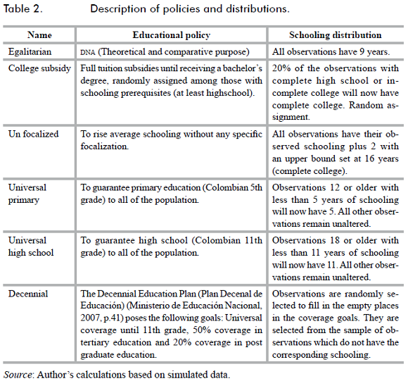
According to what has been stated so far, 6 schooling distributions are built in order to represent as many educational policies. One of them (egalitarian) does not represent a feasible educational policy. It is relevant, though, as a comparison and purely theoretical scenario. The remaining five share a basic characteristic, beside their feasibility: compared to the observed schooling distribution for 2004⁹, all of them are strictly better in a Pareto sense¹⁰. Since the schooling distributions are built from the observed one, no individual is allowed to "loose" schooling years. Table 2 presents the educational policies and their corresponding schooling distributions. The column named distribution includes a brief description of each one and the way it was built. Figure 4 shows histograms of all of the schooling distributions.

2. Descriptive statistics

The selection of these policies attempts to include a wide range of possibilities, based broadly on their variance and the section of the density where most of the changes occur. Thus, egalitarian has no variance. College subsidy, on the other hand, has a very large one. Unfocalized makes the same (absolute) changes throughout the distribution. Universal primary focuses on the lower section, universal high school on the center and decennial on the upper section.

Table 3 presents some descriptive statistics of the counterfactual schooling distributions, as well as the one observed in the 2004 data. All of the distributions but egalitarian have a higher mean than the observed one, which goes from 9 (egalitarian) to 13.7 (decennial). Standard deviation has a broader range, going from 0 (egalitarian) to 4.57 (college subsidy). Gini coefficient for the counterfactual schooling distributions is very different between them and is consistent with the policy selection mentioned above.

3. Labor earnings function

Table 4 shows the most important coefficients of the Mincer equations, estimated with the 2004 data. These estimations have a purely statistical relevance in this paper. Thus, the only interpretation for these parameters is as marginal effects on the simulated labor earnings. Since potential experience remains unaltered throughout the different distributions, the corresponding coefficients are irrelevant at this point.

Each additional year of schooling will generate 7% more labor earnings, if the individual is a woman, and 5%, if he is a man. If that additional year takes the individual to "finish" high school, earnings would rise approximately 15% (for both genders). If he/she "finishes" college, labor earnings would be 52% larger (exp 0.048+0.37) in the case of men, and 73% (exp. 0.07+0.48) in the case of women.

Although the results are not reported, the Mincer equations are estimated with the 1985 and 1995 data, too. The schooling coefficient is close to the one reported in papers with similar data and specifications (i.e. Núñez and Sánchez, 1998a).

B. Results

Table 5 shows mean labor earnings, Gini coefficient and Theil index for each of the counterfactual earnings distributions, as well as the corresponding standard errors. Table 6 ranks the distributions according to these criteria. A lower number in this ranking means a lower value in the results in table 5. Figure 5 shows the results in terms of inequality (Gini and Theil).

Even though the fit of the labor earnings function is good (the adjusted R -squared is somewhere near 50% in both cases), it is responsible to focus the analysis on comparative rather than absolute results. Thus, the main, but not only, element of analysis is the comparison between the counterfactual scenarios in terms of inequality, which, according to what has been stated in previous sections, is equivalent to establishing a comparison between the educational policies in this particular dimension.

As it could have been expected, the distribution with the lower inequality is the one that comes from the simulation of the egalitarian distribution. It is also illustrative, though predictable, to see that egalitarian has the worst results in terms of mean earnings. Even if it is beyond the scope of this paper, it is important to underline the possible trade off between the reduction of inequality and the level of labor earnings.

Universal high school is the best plausible policy in terms of inequality. Since this is a very similar policy, though a more ambitious one, to what was observed in Colombia during the last years (recall figure 3), an optimist interpretation would be that what has been done would yield good results in the long run¹¹. On the other hand, the earnings distribution resulting from the college subsidy policy is the most unequal one. Although this is somehow expected, it is very important in terms of policy design. Since there is a large amount of empirical evidence about the relevance of high skilled (college educated) wages in explaining the rise in inequality observed in the last decades, it is not unlikely that similar policies to this one could initially be thought of as equalizing ones. As it has been shown, this is definitively not the case. Thus, it could be concluded that investing in high qualification alone would lead to higher inequality, while doing so in medium qualification lead towards the opposite.

One of the most interesting results is the relative position of decennial. Right behind universal high school, it is the second best of the plausible policies. This is relevant for several reasons. First, decennial is a quite disperse schooling distribution when the variance is used as a measure of dispersion. Second, the mean of the resulting earnings distribution is the highest, contradicting the possible trade off between level and inequality in labor earnings. Thus, by equalizing opportunities and high levels of investment in generating skilled labor, decennial achieves good results in terms if labor earnings inequality without any sacrifice in their level. Given the large earnings differential between skilled and unskilled labor, the ambitious goals in terms of tertiary education coverage lead to interesting results in term of inequality. It is straightforward to see why this raises mean earnings as well.

Comparing this last result to the opposition between college subsidy and universal high school leads to a very important policy implication.

Since decennial implies a large investment in high skilled labor, full coverage in high school and just a small rise in inequality compared to universal high school, the results suggest that large investments in tertiary education could be made without large increases in inequality if high school coverage is previously guaranteed.

Base on all of the above, a very preliminary comparison between two different paths towards a larger proportion of high skilled labor force can be posed. If universal primary is taken as a starting point, and a higher proportion of high skilled labor is taken as the final target, one path would be going straightly from one to the other (college subsidy). The other path would introduce an intermediate stage: full high school coverage. Thus, the resulting distribution would be decennial. Based on the already mentioned results in terms of Gini coefficient, the second "path" would be definitively better than the first one.

The un-focalized policy, as one could have expected, lands right in the middle of all of the rankings. This is quite interesting, though, since it highlights the importance of thinking about educational policy and the implications of the composition of the schooling distribution on the labor earnings distribution. It reinforces the assumption that composition does matter.

Finally, universal primary seems to make no reduction in inequality when compared to the observed one. The difference between their Gini coefficients, for example, is very small in magnitude and not statistically significant if confidence intervals are built around them. Nevertheless, since it is embedded in universal high school and decennial, it is not to be thought of as irrelevant.

C. The participation effect

The results presented in the last section did not take into account the effect of the educational policies on labor force participation. As it was already mentioned, since schooling is involved in an individual's decision of whether or not she participates in the labor market, educational policies could affect those decisions. Nevertheless, these effects were not included because doing so would require the unlikely and strong assumption that all of the increases in participation, no matter their magnitude, could be perfectly absorbed by the labor market.

Results in tables 5 and 6 rest on an equally strong assumption: participation remains unaltered by educational policies. Therefore, it is important and necessary, for comparison purposes, to present the results that are obtained when the participation effect is included. These can be found in tables 7 and 8, which are analogous to tables 5 and 6.

Several points are worth noting. First, comparative results are identical. Nevertheless, the results are clearly weaker, in magnitude, when the participation effect is included. The distribution under which inequality is lower is still egalitarian with a Gini coefficient of 0.45, which strongly differs from the original 0.28 in table 5. The range of the new Gini coefficients is also narrower, making most of the differences between policies not significant form a statistical perspective.

All of these can be basically explained by the positive marginal effect of schooling in the participation equation. Many individuals who do not participate in the historical data will end up doing so in the coun-terfactual scenarios, and this will be more frequent in the lower part of the schooling distribution. Furthermore, since these individuals are also more likely to be in the lower part of the earnings distribution, inequality rises.

Thus, the inclusion of the participation effect generates less variation among the resulting labor earnings distributions and higher overall inequality. The relative results do not change, though. Since the two assumptions (perfect absorption and constant participation) can be interpreted as the two extreme situations among an infinite range of scenarios, the comparison between policies appears to be very robust.

D. Robustness checks

Table 9 summarizes the results of some robustness checks¹².One could think of the results being driven by two kinds of unwanted elements: the year of the data (particular context) from which the earnings and participation equations are estimated and the specification of the Mincer equation. Thus, the whole estimation and simulation process was repeated with four different variations. First, the earnings functions were estimated with 1985 and 1995 data. These years were selected in order to estimate the Mincer equation before (1985) and during (1995) the period of rising inequality in Colombia. The policy rankings, according to the Gini coefficient, are presented on columns 2 and 3 of table 10. Column 4 shows the results when age is included instead of potential experience in the earnings function. Finally, the results after including schooling levels instead of the schooling years and level premia in that same equation can be found in column 5. In order to allow an easy comparison, original results (from table 6) are included in column 1.

As it can be observed, comparative results are extremely robust. Not only they remain unaltered when the participation effect is included, but the same happens when the already mentioned changes are introduced in the estimation of the Mincer equation. The only case in which something different is obtained is when schooling levels are included instead of schooling years and premia in the Mincer equation. In this case, universal primary ranks 4^th, moving unfocalized to he 5^th position. This happens because all of the changes in universal primary lead to a change in schooling level, while most of the changes in unfocalized don't. Furthermore, the estimated inequality for these two policies was not different, from a statistical point of view, under the baseline estimation (table 5). Thus, nothing can be said about their position (relative to each other) from these exercises.

It is absolutely necessary to make explicit some of the limitations of the methodology that has been used. First, it is an absolutely static one. The way in which the participation decision is modeled, as it was widely discussed, is extremely simple. These led to unrealistic changes in participation decisions under some of the policies evaluated. For these reason, the main results were presented without the participation effect. Second, these policies would have very different costs, which have to be taken into account in policy design. This will be addressed in basic and preliminary way in the following section. Finally, as it has already been discussed, no General Equilibrium effects have been included in the simulation exercises. A brief discussion regarding this topic can be found in section VII.

E. Policy costs

Table 10 presents a very general estimation of the cost of each of the plausible policies under comparison (Column 1). These estimates are obtained using average costs for one year in primary, secondary and tertiary education found in the literature (Barrera and Dominguez, 2006; Plan Nacional de Desarrollo 2002-2006) and adjusting the total cost to a population of 40 million with a starting schooling distribution as the one observed in 2004. This means that policies are valued under many assumptions, two of which are necessary to make explicit. First, this is a one-time cost associated with the transition from the actual schooling distribution to the objective one. In practice, costs would be paid for during several years and would also include the costs of maintaining the educational system¹³. Second, these costs are calculated under the assumption that this would all be publicly financed, which needs not to be the most efficient way.

Column 2 includes the difference between the fitted Gini and the estimated one for each policy (from table 5), which is a quantitative measure of the reduction in inequality achieved under each one of the policies. With these differences and the total costs from column 1, the cost per unit of reduction in the Gini Index is estimated (column 3) for those policies that actually reduce inequality. These estimates can be thought of as a measure of efficiency in inequality reduction under each policy. Universal high school comes up as the most efficient one, adding up to its dominance over the other policies. About decennial, since universal high school is embedded in this policy and has a lower estimated Gini, it is obvious that costs per unit of reduction will be a lot higher. Un-focalized, once again, provides obvious but important information: rising average schooling without any focus is inefficient.

It is worth noting at this point that these costs do not include one of the most important consequences of the educational policies. Since aggregate human capital is being raised under all of these policies, it is likely that this would have effects o aggregate production, tax revenue, etc. and all of these would depend greatly on the particular composition of each one of the schooling distributions. Some intuition on these un-included effects can be drawn by the large differences in mean labor income for each simulation (table 5).

VII. General equilibrium effects: brief discussion

One of the main drawbacks of the methodology that has been used in paper is its lack of capacity to include General Equilibrium (GE) effects. Nevertheless, the work that has attempted to include GE effects has shown that the results in this framework are not that different from the ones obtained in a partial equilibrium one¹⁴.

Some of the robustness exercises presented in section VI can be used to support the claim that comparative results, which are the focus of this paper, would probably be robust to GE effects. Among the many ways in which GE effects could affect these results, two are the most straightforward to think of: labor supply and wages. About the first, it has been shown that, although quantitative results are deeply affected by different assumptions on the effects of schooling distribution changes on labor force participation, relative results are not.

Thus, the exercises that have been carried out provide some information, at least about the robustness of the results to GE effects in the extensive margin of labor supply. Regarding wages, table 9 showed how the ranking of the different policies remained unaltered when prices for 1985 and 1995 were used instead of the 2004 ones in the simulations. The importance of these three different years is that the wage structure was totally different in each one of them. In fact, as it was discussed in Section IV, there is a great amount of empirical evidence on the changes of relative wages and their relation to changes in inequality during these periods (roughly 1980-1989, 1990-2000, 2001-today). Thus, these robustness exercises support the claim that comparative results would probably remain unaltered if GE effects in wages were included.

Nevertheless, it is important to highlight that these effects on wages would most likely have differential effects on each policy. For instance, universal primary would have little effect on the relative supplies of differently skilled workers. It would rather lead to an increase in the average schooling of low skilled labor, thus reducing (in GE ) the return to each schooling year within this qualification group. The most likely GE effect on inequality would be an increase due to the fact that wages in the lower part of the distribution would not rise as much they do in the partial equilibrium framework (there would probably be a small effect on the wages in the margin between low and medium qualification, which would go in the same direction). The GE effects on college subsidy, on the other hand, would go in the opposite direction. The more than proportional increase in high skilled labor would lead to falling high skill wages, which would affect every qualified worker and not only the ones receiving the subsidy.

Therefore, inequality would probably be lower in a GE framework, compared to this partial equilibrium one. GE effects on universal high school, would not be straightforward, although inequality under GE would most likely be higher, since low skilled workers would disappear, thus lowering the wages for a large group of medium skilled workers (the ones with fewer amounts of other types of human capital). What would happen with un-focalized and decennial would strongly depend on the degree of substitution between different types of labor and the elasticities of their relative demands.

VIII. Conclusions

Counterfactual labor earnings distributions were simulated. The only difference between them comes from the generating process, in which the schooling of individuals (hence the schooling distribution) was changed in order to represent some educational policies. A comparative analysis was established in terms of the inequality of the resulting earnings distributions. This allowed for comparison between the educational policies in this particular dimension. All of the process happens inside a partial equilibrium environment in which labor earnings are endogenous but relative prices remain unaltered.

Guaranteeing high school education to all of the population proves to be a really powerful tool in terms labor earnings inequality reduction. The results of this paper suggest that this should be done before attempting to do large investments in tertiary education coverage. When this happens, schooling distributions with relatively high variance can coexist with comparatively low levels of inequality and high mean earnings. On the other hand, failing to provide universal high school coverage before focusing on tertiary education leads to higher inequality.

There is some evidence that the magnitude of the changes in inequality produced by the educational policies seems to be strongly dependant on the characteristics of the labor market. Inequality reductions appear to be quite larger when the labor market is not able to absorb the changes in participation generated by the shifts in the schooling distribution. Although it is far beyond the reach of this paper, this could imply that educational policy has a larger effect, in terms of inequality reduction, in weaker economies (such as the ones in developing countries). Research on this is strongly encouraged by these preliminary results.

Are the results of this paper a precise prediction of the inequality that would arise from the execution of these educational policies? It would be irresponsible to say so. Nevertheless, they create useful elements for their comparison in this particular dimension, as well as they provide clues on their interdependence with other elements. The main results are extremely robust to changes in equation specification and market structure proxies such as the inclusion of participation effects or the wage structure underlying the prices used in the simulations. This allows rejecting the idea that they are driven by forces different from the educational policies and, most importantly, that the comparative results depend on the particular context or environment in which they area analyzed. Thus, what has been presented in this paper must be interpreted as an initial step in the provision of decision elements for public policy design, which has been produced through the use of a rigorous methodology. All of these should be complemented with research focusing on other dimensions of educational policy.

"The history of interest among economists in the distribution of income is as long as the history of modern economics itself" (Becker and Chiswick, 1966, p. 358). As long as inequality levels remain as high as they actually are, that interest would still exist. Educational policy is still a powerful tool in this sense. The results of this paper suggest the possibility of achieving some inequality reduction without any sacrifice in mean earnings (though probably at a very large cost). Nevertheless, educational policy is just one of the possible means to achieving a less unequal income distribution. The problem requires creative initiatives integrating simultaneous and complementary actions supported on innovative academic research.

FOOT NOTES

¹ This distribution is based on the goals included in the Colombian "Plan Decenal de Educación 2006-2015" (Decennial Educational Plan 2006-2015).

² The proportion was 27% only 8 years before.

³ DANE.

⁴ Potential experience = Age-schooling - 6.

⁵ Note that 84 hours a week is 12 hours a day x 7 days a week.

⁶ This numbers are 12,001,999 and 6,120,098, respectively, when observations are properly weighed. All of the estimations in this paper include sample weights.

⁷ Even though the methodology is proposed and applied in more general terms, it is introduced in the specific way that it operates on this paper.

⁸ This specification comes from a standard income equation y_i = R.H_i, in which R is the rental price of Human Capital and Hi is the individual stock of HC. In particular, H_i = exp(Χ_iΘ + ε) and α = ln R .

⁹ The counter factual schooling distributions are built from the observed one for 2004.

¹⁰ Under the assumption that more schooling is always preferred to less schooling or, in other words, that the marginal utility for an additional year of schooling is always positive within the relevant range.

¹¹ This result seems to be sensitive to how perfectly the objective is accomplished. For instance, when 1% desertion is allowed between high school grades, the Gini coefficient jumps to 0.34596.

¹² The participation effect is excluded in these exercises.

¹³ This could imply many externalities and feedbacks which would make any similar attempt to include them a futile one.

¹⁴ See, for example, Lee (2004) and Lee and Wolpin (2006).

References

1. BARRERA, F., and DOMÍNGUEZ, C. (2006). Educación básica en Colombia: opciones futuras de política. Bogotá, Departamento de Planeación Nacional.        [ Links ]

2. BEAUDRY, P., and GREEN, D. (2000). "Cohort patterns in Canadian earnings: Assessing the role of skill premia in inequality trends", The Canadian Journal of Economics, 33(4):907-936.        [ Links ]

3. BECKER, G. S., and CHISWICK, B.R. (1966). "Education and the distribution of earnings", The American Economic Review, 56(l):358-369.        [ Links ]

4. BOURGIGNON, F., and FERREIRA, F. (2005). "Decomposing changes in the distribution of household incomes: Methodological aspects", in Bourguignon et al. (Eds.), The microeconomics of income distribution dynamics in east Asia and Latin America (pp. 17-48). Washington, D. C.: World Bank and Oxford University Press.        [ Links ]

5. CÁRDENAS, M., and BERNAL, R. (1999). "Changes in the distribution of income and the new economic model in Colombia", Serie de Reformas Económicas, 36, Santiago, Cepal.        [ Links ]

6. DINARDO, J.; FORTIN, L., and LEMIEUX, T. (1996). "Labor market institutions and the distribution of wages, 1973-1992: A semiparametric approach", Econometrica, 64(5):1001-1044.        [ Links ]

7. HECKMAN J.; LOCHNER, L., and TODD, P. (2006). "Earnings functions, rates of return and treatment effects: The mincer equation and beyond", in E. Hanushek and F. Welch (Eds.), Handbook of the economics of education (vol. 1, chap. 7). Amsterdam, New York, Elsevier.        [ Links ]

8. JOHNSON, G. E. (1997). "Changes in earnings inequality: The role of demand shifts", The Journal of Economic Perspectives, 11(2):41-54.        [ Links ]

9. JUHN, C.; MURPHY, K., and PIERCE, B. (1993). "Wage inequality and the rise in returns to skill", The Journal o Political Economy, 101(3):410-442.        [ Links ]

10. KATZ, L., and MURPHY, K. (1992). "Changes in relative wages, 1963-1987: Supply and demand factors", The Quarterly Journal of Economics, 107(1):35-78.        [ Links ]

11. KEANE, M., and WOLPIN, K. (1997). "The career decisions of young men", The Journal of Political Economy, 105(3): 473-522.        [ Links ]

12. KEANE, M., and WOLPIN, K. (2001). "The effect of parental transfers and borrowing constraints on educational attainment", International Economic Review, 42(4):1051-1103.        [ Links ]

13. LEE, D. (2004). "An estimable dynamic general equilibrium model of work, schooling, and occupational choice", International Economic Review, 46(1):1-34.        [ Links ]

14. LEE, D., and WOLPIN, K. (2006). "Intersectoral labor mobility and growth of the service sector", Econometrica, 74(1):1-46        [ Links ]

15. MINCER, J. (1996). "Changes in wage inequality, 1970-1990" (Working Paper 5823). NBER.        [ Links ]

16. MINISTERIO DE EDUCACIÓN NACIONAL (2007). Plan Decenal de Educación 2006-2016. website: http://www.plandecenal.edu.co/html/1726/articles-166057_cartilla.pdf. Consulted on 07/22/2010.        [ Links ]

17. MURPHY, K.; RIDDELL, W. C., and ROMER, P. (1998). "Wages, skills, and technology in the United States and Canada" (Working Paper 6638). NBER.        [ Links ]

18. NÚÑEZ, J. and SÁNCHEZ, F. (1998a). "Educación y salarios relativos en Colombia, 1976-1995: determinantes, evolución e implicaciones para la distribución del ingreso", Archivos de Macroeconomía, 74. Bogotá, Departamento Nacional de Planeación.        [ Links ]

19. NÚÑEZ, J., and SÁNCHEZ, F. (1998b). "Descomposición de la desigualdad del ingreso laboral urbano en Colombia:1976-1997", Archivos de Macroeconomía, 86. Bogotá, Departamento Nacional de Planeación.        [ Links ]

20. NÚNEZ, J., and SÁNCHEZ, F. (2002). "A dynamic analysis of household decision making in urban Colombia, 1976-1998", Archivos de Macroeconomia, 207. Bogotá, Departamento Nacional de Planeación.        [ Links ]

21. PLAN NACIONAL DE DESARROLLO 2002-2006. República de Colombia.        [ Links ]

22. PERACCHI, F. (2006). "Educational wage premia and the distribution o f earnings: An international perspective", in E. Hanushek and F. Welch (Eds.), Handbook of the Economics of Education (vol. 1, chap. 5). Amsterdam, New York, Elsevier.        [ Links ]

23. SANTA MARÍA, M. (2004). "Income inequality, skills and trade: Evidence from Colombia during the 80s and 90s", Documento CEDE 2004-02. Bogotá, Universidad de los Andes.        [ Links ]

24. VÉLEZ, C.E.; LEIBOVICH, J.; KUGLER, A.; BOUILLÓN, C., and NÚNEZ, J. (2005). "The reversal of inequality trends in colombia, 1978-1995: A combination of persistent and fluctuating forces", in F. Bourguignon, F. Ferreira and N. Lustig (Eds.), The microeconomics of income distribution dynamics in east Asia and Latin America (pp. 125-174). Washington, D. C., World Bank and Oxford University Press.        [ Links ]