DOI: 10.13043/DYS.73.2

Fiscal Policy in a Small Open Economy with Oil Sector and non-Ricardian Agents¹

Política fiscal en una economía pequeña y abierta con un sector de petróleo y agentes no-Ricardianos

Andrés González²
Martha López³
Norberto Rodríguez⁴
Santiago Téllez⁵

1 We thank Hernando Vargas, Eduardo Sarmiento Gómez, Jesus A. Bejarano and Sergio Ocampo for comments on earlier drafts. We also thank Guilherme de Almeida Bandeira for early research assistance in the model. The views expressed in the paper are those of the authors and do not represent those of the Banco de la República or its Board of Directors.

2 Associate Professor, Universidad de los Andes. Bogotá, Colombia.

3 Researcher, Research Unit, Banco de la República, Bogotá, Colombia, corresponding author, mlopezpi@banrep.gov.co.

4 Principal Econometrician, Department of Macroeconomic Models, Banco de la República. Bogotá, Colombia.

5 Economist, Department of Macroeconomic Models, Banco de la República. Bogotá, Colombia.

Este artículo fue recibido el 18 de febrero de 2013; revisado el 3 de septiembre de 2013 y, finalmente, aceptado el 14 de abril de 2014.

Abstract

In this paper we develop a dynamic stochastic general equilibrium fiscal model for the Colombian economy. The model has three main components: the existence of non-Ricardian households, price and wage rigidities, and a fiscal authority that finances government spending partly with public debt. The model is calibrated to capture the empirical evidence on the macroeconomic effects of government spending and it is used to study the effect of an oil price shock under different fiscal policy rules. Our results show that fiscal multipliers in Colombia are positive in a way consistent with the evidence. Our analysis also shows that a structural fiscal rule delivers a better outcome in terms of macroeconomic volatility relative to a balanced budget rule or a countercyclical fiscal rule.

Key words: Fiscal multipliers, fiscal policy rules, non-Ricardian households, DSGE model.

JEL classification: D91, E21, E62.

Resumen

En este artículo planteamos un modelo fiscal de equilibrio general dinámico y estocástico para la economía colombiana. El modelo tiene tres componentes principales: a) la existencia de hogares no-Ricardianos, b) rigideces de precios y salarios y c) una autoridad fiscal que financia su gasto en parte con deuda pública. El modelo se calibra para capturar la evidencia empírica de los efectos macroeconómicos del gasto del gobierno y a su vez es usado para estudiar el efecto de un choque de precios del petróleo con diferentes reglas de política fiscal. Nuestros resultados muestran que los multiplicadores del gasto en Colombia son positivos de acuerdo con la evidencia. Nuestro análisis también muestra que en términos de disminución de la volatilidad macroeconómica, una regla fiscal estructural es preferible a una regla de presupuesto balanceado o una regla fiscal contracíclica.

Palabras clave: Multiplicadores fiscales, reglas de política fiscal, hogares no-Ricardianos, modelo DSGE.

Clasificación JEL: D91, E21, E62.

Introduction

Macroeconomic stability is one of the key ingredients to enhance economic growth. Nonetheless, the development of a more integrated world during the last couple of decades has put forward the need to introduce more instruments to achieve this elusive goal. In this sense, not only monetary policy has a role but also fiscal policy has gain relevance as an important element for overcoming macroeconomic instability. This is true for both developed and emerging market countries.

In the particular case of small open economies characterized by endowments of natural resources, such as oil, very often their economies are affected by shocks that result not only in the so called Dutch disease but also in economic volatility. Another characteristic that might reinforce this instability, in some of these economies, is the presence of great proportion of agents that do not have access to capital markets to smooth consumption (non-Ricardian agents). These consumers, who receive transfers coming from higher oil revenues, consume all their disposable income period by period, which contributes to macroeconomic volatility.

Colombia is one example of this kind of small open economies with a significant size of credit constraint households and oil revenues. Even though its GDP has been growing at a positive rate, the economy as a whole has showed high economic instability since 2004. The rise in oil prices during the last decade resulted in large capital inflows coming from foreign direct investment (FDI) as a percentage of GDP (particularly in the oil sector). FDI increased 4.0% between 2004 and 2011 compared to 2.2% between 1993 and 2003 (Garavito, Iregui and Ramírez, 2012). The exchange rate presented a real appreciation of 30% between 2004 and 2011. The ratio of credit to GDP increased from 46.1% in 2004 to 67.7% in 2008. Something similar occurred with asset prices, whose real index went from 140.0 to 416.4 in the same period. Finally, economic growth went from 3.5% in 2005 to 7.5% in 2007 and slowed down to 0.1% during 2009; but the bubble remerged fueled by capital inflows in 2011.

The fiscal authority might have a tool to contribute in stabilizing the business cycle: a fiscal rule that saves part of oil revenues during booms and that spends excess revenues during bad times may reduce output volatility. As we will show in the paper, a fiscal policy rule enables the government to smooth consumption of non-Ricardian agents dampening the business cycle. In addition, these rules constitute another instrument, besides the policy interest rate, that allows policy-makers to achieve macroeconomic stability.

In order to be able to evaluate different fiscal rules, first we need to develop a fiscal model that describes important aspects of the Colombian economy. In particular, the model should capture the fact that in Colombia (like in many other countries) consumption increases after a government spending shock. In this paper we develop a dynamic stochastic general equilibrium fiscal model for the Colombian economy that replicates this fact. The model has three main components: the existence of non-Ricardian households, price and wage rigidities, and a fiscal authority that finances public spending partly with public debt and partly with taxes and oil revenues (see Colciago, 2011; Galí, López-Salido and Vallés, 2007; Monacelli and Perotti, 2010). The intuition behind this set up is clear. Introducing non-Ricardian agents is equivalent to making part of the aggregate demand independent of the real interest rate which allows these consumers to overcome wealth effects. A necessary condition for private consumption to increase is for the real wage to increase. At the same time, a positive response of real wage requires labor demand to shift out. This happens in our model because of rigidities in price setting by monopolistically competing firms: "When government spending increases, firms face an outward shift in the demand curve for the variety they produce; those firms that cannot change their prices meet this extra demand by increasing production, hence shifting out the derived demand for labor" (Monacelli and Perotti, 2008). In addition, if the government finances government spending partially with public debt, consumption of non-Ricardian consumers will not fall as long as taxes are collected sufficiently slowly.

The objective of the paper is to use the model to show how the Colombian economy would benefit in terms of welfare and less macroeconomic volatility if the government decides to use a fiscal rule that saves part of the oil revenues in the form of reduced debt. This kind of fiscal rule is known as a Structural Surplus Rule (SSR) and has been implemented in countries like Chile and Norway (see Pieschacón, 2012). We compare this rule with a benchmark rule called a Balanced Budget Rule (BBR), which is highly procyclical in terms of increasing government spending when there are excess revenues of oil. This benchmark rule resembles very much what has been the fiscal policy in Colombia with respect to the government's management of oil revenues until now (see Lozano and Toro, 2007). As a complement, we also analyze what happens if the government decides to implement a countercyclical rule (CCR) in which the policy instruments represent strong automatic stabilizers. In addition, we analyze the interaction between fiscal and monetary policy in terms of welfare. We want to answer if the implementation of a SSR contributes to a less aggressive monetary policy stance when the economy faces a shock in oil prices.

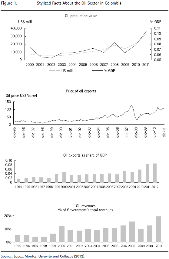
Moreover, the data strongly suggests the growing importance of the oil sector in recent years in Colombia. As we can see in figure 1, oil prices increased notoriously and oil production as a percentage of GDP has increased since 2002. Exports to GDP ratio achieved a level of 8.6 percent in 2012. And more importantly, government's oil revenues reached a 19.3 percent of total revenues in 2011.

The rest of the paper is organized as follows. Section one presents empirical evidence on the effects of government spending in the Colombian economy. Section two describes the model. In section three the parameter values are discussed. Section four provides the simulations of the model to shocks in government spending and to oil prices as well as welfare analysis for the different kind of rules. Finally, section five concludes.

I. Empirical Evidence

In this section we document the effects of government spending shocks on key macroeconomic variables. Following Vargas, Gonzalez and Lozano (2012) we identify the government spending shock with a method that meets the criteria of no anticipation and no contemporaneous correlation with output. To do so, we define the shock as the difference between the Central Government actual primary expenditures (overall spending without interest payments on public debt) and the forecast made of this variable. Next we consider the effect of the shock in a VAR. We use quarterly data for the 1999 to 2011 period. In order to examine the effect on a number of variables, without including too many variables in the VAR, we follow Ramey (2011) s' strategy of using a fixed set of variables and rotating other variables of interest. The fix set of variables consists of the no anticipated spending shock, the log of real per capita government spending, and the log of real per capita GDP. The series of variables that we rotate, one at a time, are private consumer expenditure, total hours, real wage, real exchange rate and net exports as percentage of GDP. Four lags of the variables and a linear trend are used.

Figure 2 shows the results. The impulse responses to a shock in the no anticipated government spending shock have been normalized so that the response of government spending is equal to one. Besides, to obtain the implied government spending multiplier, we use the corresponding ratio of GDP to government spending, 6.7 during the period. We report 68% confidence intervals as used commonly in this kind of studies. In response to the fiscal expansion, we observe an increase in both output and consumption peaking three quarters after the shock. The peak of the implied government spending multiplier ranges between 0.7 and 1.8. This range is in line with a study by Blanchard and Leigh (2013) for the IMF. Their estimates of fiscal multipliers for other economies have been between 0.9 and 1.7. The increase in private consumption is also in line with many other SVAR studies on the effects of government spending. See, for example, Ravn, Schmitt-Grohé and Uribe (2007) and Mountford and Uhlig (2009). The size in consumption multiplier points to the importance of that variable in the effect of government spending on output, suggesting the presence of non-Ricardian effects. In addition, cumulative multiplier reaches a value of 3.3 at a four quarter horizon. The empirical evidence is similar to that found by Lozano and Rodríguez (2011) and Restrepo and Rincón (2006) for the case of Colombia.

Figure 2 also shows that real wage increases in response to the shock. The effect on total hours is ambiguous; the expansion in public spending results in deterioration in the current account and the real exchange rate appreciates. Other studies also find this kind of results for other economies, see, for example, Monacelli and Perotti (2010), Ravn et al. (2007) and Ramey (2011).

II. Model

This section presents a model that replicates most of the empirical evidence presented in the previous section and that can be used for fiscal policy analysis regarding fiscal policy rules when the economy is facing oil prices shocks. The model developed is along the lines of Galí et al. (2007) and Kumhof and Laxton (2009). From the Galí et al. (2007)'s approach, our model shares that it is a DSGE New Keynesian model with non-Ricardian agents which suits very well the Colombian economy given the high proportion of credit constraint households in the economy (near 80 per cent according with our calculations). From the Kumhof and Laxton (2009)'s approach we take into account how they model the different fiscal policy rules. Some additional characteristics of the model, specific to the Colombian economy, are that we take into account that we are dealing with a small open economy and that we have oil income as an important source of government revenue.

A. Households

We assume that there is a fraction Γ of Non-Ricardian households in the economy whose variables are denoted by N and a fraction (1-Γ) of Ricardian agents whose variables are denoted by R. The utility function of households is non-separable between consumption and labor.

1. Ricardian Households

Ricardian Households, denoted by R, are indexed between Γ and 1 and have preferences of the form

where c_R,t is a consumption index and n_R,t are hours worked. The parameter σ_R measures the intertemporal elasticity of substitution, θ_R is a scale parameter and λ_R the inverse of the Frisch elasticity. This kind of preferences was introduced by Greenwood, Hercowitz and Huffman(1988) (GHH) and have the property that the wealth effect on labor supply is muted. As we will see in the results, GHH preferences and price rigidities allow the increase of consumption as a response to an increase in government spending. The term outside the braquet corresponds to part of the CRRA utility function.

These households maximize utility subject to two constraints. First their budget constraint is given by

The left hand side of the equation represents purchases in consumption including taxes, after subsidy net investment, and purchases of domestic and foreign assets, where following Schmitt-Grohé and Uribe (2003), the foreign interest rate , depends on the country's net foreign asset position, b_t^* as a percentage of GDP, the real exchange rate and an exogenous risk premium shock, φ_b. The terms in the right hand side represent sources of income including after tax labor income, after tax holdings of capital, domestic nominal discount bonds issued by the government, foreign bonds holdings, profits from unions and intermediate firms, and ξ_t^h, respectively, and lump-sum net transfers.

The second constraint is given by the capital accumulation equation

where the investment, x_t, exhibits adjustment costs.

2. Non-Ricardian Households

Non-Ricardian Households, denoted by N, are indexed between 0 and Γ and solve a similar problem but they are assumed to have no access to financial markets. Therefore, they consume period by period all their labor income and the transfers received from the government. They seek to maximize their lifetime utility

subject to the budget constraint

where the left hand side corresponds to after tax consumption and the right hand side to after tax labor income, dividends from unions and lump sum transfers.

B. Domestic and Imported Consumption and Investment

It is assumed that the composition of the consumption bundle is identical for both types of households; therefore we will not use the subindex for household type. The consumption bundle takes the form

where c_t is a CES index that includes domestic and foreign goods, with parameter α_c determining the degree of openness and η_c the elasticity of substitution between domestic and imported goods. The lagrange multiplier, p_t^c, denotes the consumption price index that normalizes every price index of the economy as follows

As for consumption, the investment bundle x_t aggregates domestic and foreign investment according to the next function

here the Lagrange multiplier, p_t^x, indicates the investment price index. The investment good relative price is given by

where α_x represent the participation of foreign goods in investment and η_x is the elasticity of substitution between home and foreign investment goods.

C. Labor Agencies, Unions and Wage Setting

In order to introduce nominal rigidities in wages and to facilitate the aggregation, we expand the framework of Kumhof and Laxton (2009). The setup is as follows: Ricardian and non-Ricardian households sell labor to specific Ricardian and non-Ricardian unions respectively that differentiates it. Since they produce differentiated labor, these unions have monopolistic power. After buying labor from the households, the differentiated labor is sold to Ricardian and non-Ricardian agencies in perfect competition that "pack" the labor into composites of Ricardian and non-Ricardian labor respectively. Finally, both types of "packed" labor are bought by a national agency that aggregates them into a final composite to be sold to intermediate good firms.

1. Labor Agencies

As mentioned before, there are three types of labor agencies: Non-Ricardian, Ricardian and aggregate labor agency. The first two are identical and are designed to buy the differenciated labor from Ricardian, u_R,t, and non-Ricardian, u_N,t, unions to aggregate into Ricardian and non-Ricardian indexes. The national labor agency aggregates Ricardian and non-Ricardian labor "packed" by specific labor agencies and sells it to intermediate good firms subject to a CES aggregator

so that the demand for "packed" Ricardian and non-Ricardian labor are given by

with the Lagrange multiplier equal to v_t

where stands for the real wage paid by the intermediate good firms as shown below.

Non-Ricardian labor agency demands labor from union j given the aggregate labor agency's demand and the aggregation function

Thus, the demand for labor from union j is given by

where u_n,t, is the labor demanded by the national agency in equation (4). The corresponding wage index is

Aggregating over unions, we obtain the aggregate labor supplied by non-Ricardian households

where

In the same way, there is a Ricardian Labor Agency that solves a similar problem with respect to the labor supplied by Ricardian labor Unions.

2. Labor Unions

There is a continuum of unions j [0,1] that buy labor from non-Ricardian Households at w_N,t and sell it to the non-Ricardian labor agency at v_N,j,t. They have monopolistic power and can set v_N,j,t optimally with probability (1- ε) each period. Between re-optimization periods we allow the nominal wage to be adjusted according to the following indexation rule

Every union j maximizes benefits subject to this indexation rule and the demand from the non-Ricardian labor agency given by (6).

As for labor agencies, the Ricardian unions solve a similar problem to that of non-Ricardian unions.

D. Domestic Good Firms

We assume a continuum of monopolistically competitive firms producing differentiated intermediate goods. The latter are used as inputs by a (perfectly competitive) firm producing a single final good.

E. Final Good Firms

The final good is produced by a representative, perfectly competitive firm with a constant returns technology

where y^h_z,t, is the quantity of intermediate good z used as an input and θ^h > 1. Profit maximization, taking as given the final goods price p_t^h and the prices for the intermediate goods p^h_z,t, all z [0,1], yields the set of demand schedules

as well as the price index

F. Intermediate Good Firms

There is a continuum of intermediate good firms, z [0,1], with technology described by

where k_z,t and n_z,t represent the capital and labor services hired by firm z. Firms minimize cost subject to (8). The resulting real marginal cost is (note that because all firms have the same cost, we drop the z index)

G. Optimal Price-Setting

Intermediate firms are assumed to set nominal prices according to the stochastic time dependent rule proposed by Calvo (1983). Each firm resets its price with probability 1- ε^h each period, independently of the time elapsed since the last adjustment, setting price p_z^h. In absence of reoptimization, the firm follows an updating rule

H. Government

1. Monetary Policy

Monetary policy follows a conventional simple policy rule where interest rate is set by the Central Bank according with

where long-run interest rate is , the inflation target is and the feed-back parameter (the response of the policy interest rate to deviation of inflation from target) is ρ_π.

2. Fiscal Policy

The government purchases both domestic and foreign goods. These purchases are assumed to have null effect on private utility or productivity. Again, the government bundle of goods G_t is a CES aggregator of domestic and imported government purchased goods

with the Lagrange multiplier equal to p_t^G. The government goods relative prices are given by

where α_G represent the participation of foreign goods in government spending and η_G is the elasticity of substitution between home and foreign government goods.

In addition, the government taxes consumption, labor income and capital, subsidizes investment, transfers resources to Non-Ricardian and Ricardian households and issues debt in the domestic economy. The government budget constraint takes the following form

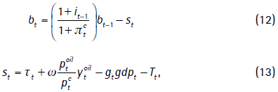
where s_t is the primary surplus and τ_t denotes the total tax revenues, the international price of oil p_t^oil* is assumed to follow an exogenous autorregresive process, implying a domestic oil price ; in the same way, oil production y_t^oil is assumed to be exogenous. ω denotes the share of oil production that the government owns, so that a fraction ω of oil revenues accrues to the government, whereas the remaining share of oil revenues go to foreign companies. The term represents goverment spending as a percentage of GDP, and T_t lump-sum net transfers.

Total tax revenues correspond to collected taxes on consumption, capital and labor income minus subsidy on investment

Government surplus gs_t is defined as

which equals the primary surplus and net interest payments on government debt. The share of government expenditure to real GDP of the economy, g_t, is assumed to follow an exogenous and autorregresive process

where is the long run government share and ρ_G captures the persistence of the process.

Similarly, tax rates on wages, consumption, holdings of capital and the investment subsidy are allowed to vary according to

where _i corresponds to _w, _k, _c and _x: the long-run tax rates, ρ_τi corresponds to ρ_τw, ρ_τk, ρ_τc and ρ_τx which represent persistency and _τi corresponds to _τw, _τk, _τc and _τx which are i.i.d. white noise shocks.

The final component of fiscal policy is the policy rule that is explained in the next section.

I. Fiscal Policy Rules

A general form of fiscal policy rule has the form

where ^rat is a structural surplus target. In Colombia in July 2011 was introduced a fiscal rule where the structural surplus target for the year 2014 is -2.3%. The remaining items correspond to cyclical adjustments according to excess tax revenue, excess revenue from mining sector and an additional debt gap variable.

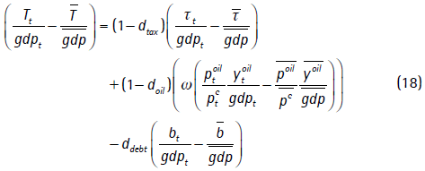
When d_tax = d_oil = d_debt = 0 holds, the rule corresponds to a strict Balanced Budget Rule (BBR) that is highly procyclical because it calls for higher spending in a boom. This has been the case in Colombia during the last decade. The case of parameter values of d_tax = d_oil =1 and d_debt = 0 corresponds to a Structural Surplus Rule (SSR) where the rule ties government spending to structural/permanent government revenues. This kind of rule has been used in countries like Chile (see Céspedes Fornero and Galí, 2012) and Norway (see Pieschacón, 2012). In this case, as mentioned before, total government spending (including interest payments) plus a time varying "surplus target" must be equal to structural revenues. In this rule, excess revenues from oil or tax revenue are saved in the form of reduced debt or increased assets. According to Céspedes et al. (2012), in the case of Chile "the idea was to acknowledge that public debt was at a level higher that was considered appropriate for a small open economy that faced exogenous credit constraint shocks and a given potential future pension liabilities". The structural surplus target, ^rat, is exogenous. As pointed out by Kumhof and Laxton (2009), this rule has at least two important implications. First, it has the ability to stabilize long-run debt. Equation (15) shows that a SSR anchors the long-run debt to GDP ratio, , which in the case of Colombia with a nominal growth rate g of 5 percent and surplus target of -2.3 percent of GDP would imply a long-run debt to GDP ratio of about 12 percent compared to the actual 30 percent level. The second implication is related to the business cycle stabilization and volatility of fiscal instruments. We will discuss this aspect in the results of the simulations of the model.

In the other extreme we have a countercyclical fiscal rule. This kind of rule corresponds to the case of a parameter value of d_tax >1 which calls for higher tax rate (or lower spending) in a boom. This rule would represent strong automatic stabilizers, such as progressive taxation or countercyclical transfers, for example unemployment insurance (Kumhof and Laxton, 2009).

In order to achieve objective of the targeting rule the fiscal authority has six instruments, three taxes τ_c,t, τ_l,t and τ_k,t, a subsidy τ_x,t, and two spending items T_t and G_t. The default instrument for our baseline results is transfers T_t . In this case, the fiscal rule is given by

where the overlined variables denote their steady state values, so that the fiscal rule activates when the variables of interest of the government deviate from their steady state values and has been set to satisfy the structural surplus budget.

J. Rest of the World

Foreign demand of home produced goods c_t^h* is given by

where the parameter µ represents the price elasticity of exports.

K. Equilibrium and Aggregation

Market clearing condition for capital, given that only Ricardian agents engage in capital accumulation is given by

Similarly for other asset holdings we have

Agregate consuption and investment are

Domestic uses of product

Finally real GDP is

L. Aggregate Welfare

Making use of the cashless limit assumption, the period utility of representative l household at time t is given by

The expectation of welfare is

In order to have a metric for the welfare gain if Colombia could switch from the BBR that follows until now to a SSR like the one in Chile or Norway, we compute the welfare gain Ω^l as

where EW_t^l,fisc is the expectation on welfare under a given combination of fiscal rule parameters and EW_t^l,BBR is the expectation of welfare under the baseline combination, the BBR. We use second order approximation of the first order conditions of the model and the utility functions to compute welfare.

Finally, we quantify aggregate welfare by way of population-weighted average of welfare gains

III. Calibration

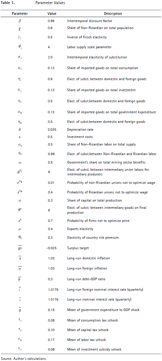
In this section we present the calibration of the model for the Colombian economy. The subjective discount factor β is set to 0.99, implying a steady state interest rate of 4%. The parameter ω is consistent with the government's share on total mining sector dividends, which corresponds to the share of government in state firm Ecopetrol. The long-run values are in line with estimates by Fergusson (2003) and Hamann, Lozano and Mejía (2011). The long-run ratio of government expenditure to GDP is 0.15 according with the data.

We also calibrated the Calvo price probability, ε^h, in 0.7 according with estimates for Colombia by Bejarano (2005) which is also in line with estimates for the United States by Smets and Wouters (2007). The Calvo wage probability was calibrated in 0.4 for Ricardian agents in line with estimates for Colombia by Bonaldi, González and Rodríguez (2011), and we assumed low wage rigidity for the non-Ricardian agents.

For the parameter Γ, share of non-Ricardian agents in the Colombian economy, we use a Superfinanciera (the banking supervision agency in Colombia) dataset recorded by each bank in the 341 form about credit card holders as a percentage of the population in working age reported by DANE (the Colombian Statistics Department): 20%. This parameter value is also consistent with Prada and Rojas (2009) who found that informal labor in Colombia is about 70% of total labor. This parameter value is similar also to the one estimated for the Chilean economy by Corbo and Schmidt-Hebbel (1991).

The elasticity of substitution among varieties of intermediate goods, θ^h, is calibrated in 6 which implies a steady-state mark-up of 20 per cent, a common value used in the literature. The inverse of Frisch elasticity was calibrated in 0.5 according with Prada and Rojas (2009). The investment cost parameter, κ, is set at 0.5 as estimated by López, Prada and Rodríguez(2009) for the Colombian economy.

The elasticity of country risk premium with respect to net foreign debt, φ_b, is set equal to 0.0024, which as pointed out by Gertler, Gilchrist and Natalucci (2003) should be small enough so that the friction in the capital market does not alter the high frequency model dynamics but nonetheless makes net foreign indebtedness revert to trend.

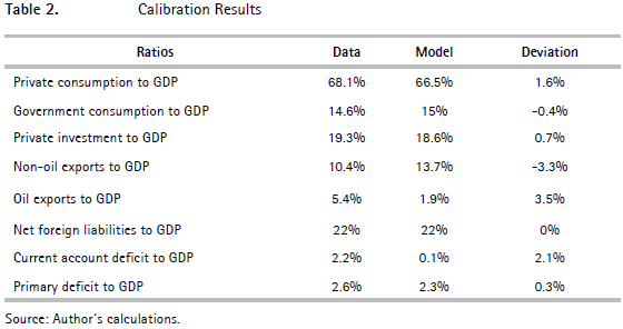
The elasticity of output to capital, α, is set to 0.3 to be consistent with the labor income share. The relative risk aversion coefficient, σ_R, was set at 2.0 according with estimates by López (2001). We fix the steady state world interest rate at 3 per cent per annum. The steady state foreign and domestic inflation rates are set at 3 per cent per annum. Table 1 summarizes all the parameters and their description. Finally, table 2 presents the different long run ratios used for the calibration along with their observed values in the data, their equivalent in the model and the corresponding percentage deviation. As can be observed, the maximum percentage deviation is 3.5%.

IV. Results

A. Comparing Predicted and Observed Impulses Responses

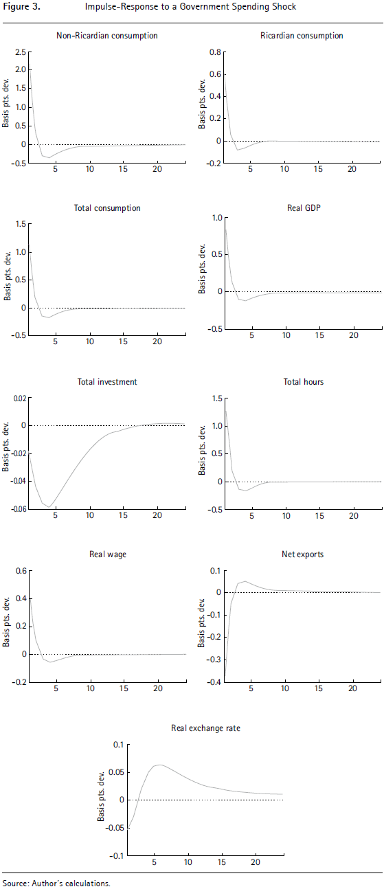
Figure 3 shows the predicted responses by the model in key macroeconomic variables to a shock in government spending. The model predicts an increase in output that implies a fiscal multiplier of 0.9, value that is in line with our empirical estimates. The model also predicts a rise in consumption of both Ricardian and non-Ricardian agents. However, the rise in consumption of non-Ricardian agents is much higher, 2.2, which allows the model to replicate the fiscal multiplier. The consumption of this group of households increase because of three facts: First, there is an expansion in hours worked as a response to the government spending shock. The demand shock under sticky prices causes output to increase and the labor demand curve shifts out. Second, the increase in labor demand causes a rise in real wages which stimulates consumption. Finally, the government spending is financed partly with public debt in such a way that in the budget constraint of non-Ricardian households the real wage increases more than taxes and consumption also rises.

Consumption of Ricardian agents also increases. Here, as illustrated by Monacelli and Perotti (2008), with GHH preferences and sticky prices consumption is higher when government spending increases. If prices are sticky, firms face an outward shift in the demand curve for the variety they produce. On the supply side, with these kind of preferences, the marginal rate of substitution between consumption and leisure is independent of consumption, then, the wealth effect is muted in the labor supply curve. But because of price stickiness, movements in the real interest rate are limited. From the Euler equation, this also limits changes in the marginal utility of consumption. In addition, under GHH preferences, consumption and labor are complements "When labor demand shifts out and hours increase along the labor supply curve, the marginal utility of consumption increases; to restore the initial value, consumption too must increase (the derivative of the marginal utility of consumption with respect to consumption is negative)" (Monacelli and Perotti, 2008).

The model also predicts an appreciation in the real exchange rate originated in the monetary policy response to the inflationary pressure. The real interest rate increases and there is a real exchange rate appreciation. As a result, the current account as a percentage of GDP deteriorates and we observe the so called twin deficit supported by the data. Finally, investment falls as a result of the increment in the real interest rate, this dampens the output response to the fiscal impulse.

B. Effects of a Transitory Shock to the Price of Oil: Comparing Different Fiscal Rules

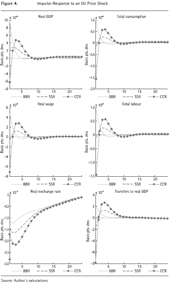
Now we turn to analyze the effects of an oil price shock on several macro variables. What the government does with the proceedings from oil depends on its fiscal policy rule. In Figure 4 we plot the impulse responses of macroeconomic variables to oil price shock of 1% for alternative fiscal policy rules. The fiscal instrument used for the comparisons is transfers T_t while tax rates and government spending are kept constant. Under a BBR (d_tax = d_debt = d_oil = 0), that is, a completely procyclical fiscal policy, the government responds to the additional oil revenue by increasing transfers to households, thus allowing (them) to increase consumption. The increase in aggregate demand generates incentives to labor demand, thus increasing wages and total hours worked. The same increase in aggregate demand generates inflation and appreciates the real exchange rate given the capital inflows. However, after four quarters output falls resulting in macroeconomic volatility and the behavior of the macroeconomic variables reverses.

In the case of a structural surplus fiscal rule, SSR, (d_tax = 1, d_debt = 0, d_oil =1), the government holds transfers relatively unchanged reducing macroeconomic volatility. Output and consumption increase but in lower amount returning faster to their steady state values that under the BBR. In this case, output increases but half the magnitude that in the case of the BBR. However, it does not fall later and its convergence is smoother than in the other two rules. We observe a similar behavior in consumption, total hours and real wage. Real exchange rate still appreciates but in a lower degree. Finally, a countercyclical rule, CCR, which implies lowering transfers to households, results in the worse scenario in terms of household's consumption. A government too conservative would cause a fall in consumption of about 4 per cent with a recovery in the third quarter almost negligible. Output would not fall as much because CPI inflation would fall and the Central Bank response would be to decrease interest rate which increases investment. Volatility under the CCR rule is as big as in the case of BBR and much higher than in the SSR. The results presented here for the BBR, which has been the rule that better resembles government's fiscal policy during the years of increase in oil prices (since 2002), are in line with the stylized facts presented in Figure 1.

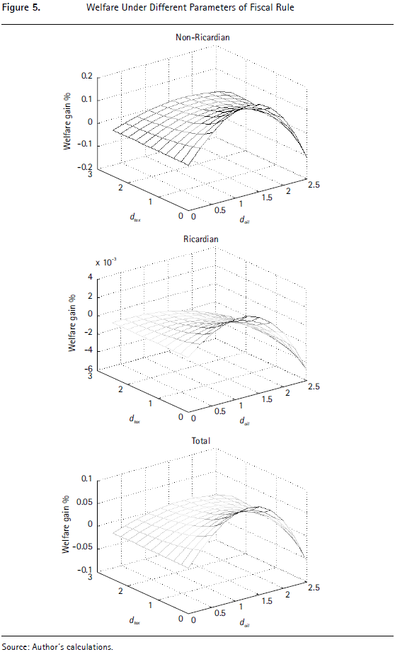
Turning to welfare analysis derived from the different fiscal rules, in Figure 5 we present different values of welfare gain, Ω, for the fiscal rule as a function of the parameters d_oil and d_tax which range between 0 and 2.5. The parameter value of d_oil = d_tax = 0 corresponds to the baseline BBR against which all parameter combination are compared. We hold the d_debt coefficient at a baseline value of zero.

The bottom subplot shows the overall welfare results. We find that welfare gains do not change very much in response to the coefficient d_tax. However, welfare gains are hump-shaped in relation to d_oil, with a maximum near 1. The corresponding welfare gain for the parameter values d_oil = d_tax = 1 are the best combination of parameter values and this corresponds to the SSR as mentioned before. In the case of a very procyclical rule, where the parameter values are close to 0, the welfare gains are low. Finally, if the fiscal authority opt for a countercyclical rule, CCR, and d_oil = 2.5 there are very steep losses.

Finally, it is also of interest to analyze whether the welfare gains are the same for the two subgroups of agents. Figure 5 also plots the welfare gain for each group of agents. There, we observe that the SSR is particularly welfare improving in the case of the non-Ricardian households, with a welfare gain of 2%, while in the case of Ricardian agents the welfare gain is almost negligible. The intuition behind this result is that in the case of the non-Ricardian households, a structural fiscal policy rule, SSR, helps to improve welfare because the government smooths consumption of non-Ricardian households when faced with an exogenous shock to oil revenues. In the case of Ricardian agents, they smooth consumption and the fiscal policy does not improve their welfare. Therefore, the presence of non-Ricardian households in the economy justifies the use of a structural fiscal rule that plays the role of a stabilizer.

C. Fiscal and Monetary Policy Interaction Under Different Fiscal Rules

In an inflation targeting regime, the monetary authority has to react to inflationary or deflationary pressures. An oil price shock pressures the general price level and the central bank has to deal with that. One of the results that we observed in the previous subsection was that the fiscal policy rule might help to stabilize the behavior of the macroeconomic variables and enhance welfare. Another question that surges is the degree to which the fiscal policy might enable the central bank to have a less aggressive monetary policy. To answer this question, we perform a welfare analysis exercise where we compare the welfare gain of a procyclical fiscal rule, a structural fiscal rule and a countercyclical fiscal rule for different values of the parameter ρ_π (the feedback coefficient of inflation in the monetary policy rule). The parameter value of ρ_π ranges between 2 (higher than one by the Taylor's principle) and 9. The baseline is a parameter value of ρ_π = 2. The results are presented in figure 6. We observe that in the case of the procyclical and the countercyclical fiscal rules the welfare gains are very high when we increase ρ_π from 2 to 6. While in the case of the structural fiscal rule a parameter value of ρ_π of 3 is enough to maximize the welfare gain. In the later, the gain from increasing the feedback parameter of inflation is not as big as in the case of a very aggressive monetary policy rules in the other two rules. This shows that under the structural fiscal rule, SSR, the monetary policy can be less aggressive in fighting inflation. It is worth noting that in the analysis, the Central Bank targets CPI inflation like is the case in Colombia.

V. Concluding Remarks

This paper presents evidence of the growing importance of government's oil revenues since the recent increases in oil prices. It also shows the importance that oil output has gain in total output and oil exports in total exports. The management of oil revenues by the government is of crucial importance for the macroeconomic performance in Colombia. In the paper, we developed a fiscal model for the Colombian economy that matches the stylized facts of a government spending shock by allowing non-Ricardian agents, price and wage rigidities and public debt.

The model was used to analyze the effects of an oil price shock in the different macroeconomic variables depending on the kind of fiscal rule that the government uses to manage oil revenues. It was shown that Colombia would benefit from implementing a Structural Surplus Rule similar to the one used in Chile or Norway to save oil revenues in the form of reduced debt, instead of being procyclical during the booms. In that case, macroeconomic volatility would be reduced and the welfare gains would be important given that this rule would help non-Ricardian agents to smooth consumption.

The paper also shows that if the fiscal authority implements a SSR, the Central Bank does not need to be aggressive in fighting inflation. The feedback coefficient on the Taylor rule would be near 3 while in the case of a BBR like the one followed until now would be around 6 in order to maximize welfare.

References

1. BEJARANO, J. A. (2005). "Estimación estructural y análisis de la curva de Phillips neokeynesiana para Colombia", Ensayos sobre Política Económica, 48:64-117.         [ Links ]

2. BLANCHARD, O. J., AND LEIGH, D. (2013). Growth forecast errors and fiscal multipliers (Working Papers 13/1). International Monetary Fund.         [ Links ]

3. BONALDI, P., GONZÁLEZ, A., AND RODRÍGUEZ, D. (2011). "Importancia de las rigideces nominales y reales en Colombia: un enfoque de equilibrio general dinámico y estocástico", Ensayos sobre Política Económica, 66(29):48-78.         [ Links ]

4. CALVO, G. A. (1983). "Staggered prices in a utility-maximizing framework", Journal of Monetary Economics, 12(3):383-398.         [ Links ]

5. COLCIAGO, A. (2011). "Rule of thumb consumers meet sticky wages", Journal of Money, Credit and Banking, 43:325-353.         [ Links ]

6. CORBO, V., AND SCHMIDT-HEBBEL, K. (1991). "Public policies and saving in developing countries" (Policy Research Working Paper Series 574). The World Bank.         [ Links ]

7. CÉSPEDES, L. F., FORNERO, J., AND GALÍ, J. (2012). Non-ricardian aspects of fiscal policy in Chile (Working Paper 663). Central Bank of Chile.         [ Links ]

8. FERGUSSON, L. (2003). Tributación, crecimiento y bienestar: el caso colombiano (1970-1999) (Documentos CEDE 003662). Universidad de los Andes, Facultad de Economía, CEDE.         [ Links ]

9. GALÍ, J., LÓPEZ-SALIDO, J. D., AND VALLÉS, J. (2007). "Understanding the effects of government spending on consumption", Journal of the European Economic Association, 5(1):227-270.         [ Links ]

10. GARAVITO, A., IREGUI, A. M., AND RAMÍREZ, M. T. (2012). Determinantes de la inversión extranjera directa en Colombia: un estudio a nivel de firma (Borradores de Economía 714). Banco de la República de Colombia.         [ Links ]

11. GERTLER, M., GILCHRIST, S., AND NATALUCCI, F. (2003). External constraints on monetary policy and the financial accelerator (Working Paper 10128). National Bureau of Economic Research, Inc.         [ Links ]

12. GREENWOOD, J., HERCOWITZ, Z., AND HUFFMAN, G. W. (1988). "Investment, capacity utilization, and the real business cycle", American Economic Review, 78(3):402-417.         [ Links ]

13. HAMANN, F., LOZANO, I., AND MEJÍA, L. F. (2011). Sobre el impacto macroeconómico de los beneficios tributarios al capital (Borradores de Economía 668). Banco de la República de Colombia.         [ Links ]

14. KUMHOF, M., AND LAXTON, D. (2009). Simple, implementable fiscal policy rules (IMF Working Paper 09/76). International Monetary Fund.         [ Links ]

15. LOZANO, I., AND RODRÍGUEZ, K. (2011). "Assessing the macroeconomic effects of fiscal policy in Colombia", Journal of Financial Economic Policy, 3(3):206-228.         [ Links ]

16. LOZANO, I., AND TORO, J. (2007). Fiscal policy throughout the cycle: The Colombian experience (Borradores de Economía 434). Banco de la República de Colombia.         [ Links ]

17. LÓPEZ, E., MONTES, E., GARAVITO, A., AND COLLAZOS, M. M. (2012). La economía petrolera en Colombia marco legalcontractual y sus principales efectos sobre la actividad económica del país (parte I) (Borradores de Economía 692). Banco de la República de Colombia.         [ Links ]

18. LÓPEZ, M. (2001). "Seigniorage and the welfare cost of inflation in Colombia", Ensayos sobre Política Económica, 39:115-131.         [ Links ]

19. LÓPEZ, M., PRADA, J. D., AND RODRÍGUEZ, N. (2009). "Evidence for a financial accelerator in a small open economy, and implications for monetary policy", Ensayos sobre Política Económica, 60(27):12-45.         [ Links ]

20. MONACELLI, T., AND PEROTTI, R. (2008). Fiscal policy, wealth effects and markups (Discussion Paper 7099). CEPR.         [ Links ]

21. MONACELLI, T., AND PEROTTI, R. (2010). "Fiscal policy, the real exchange rate and traded goods", Economic Journal, 120(544):437-461.         [ Links ]

22. MOUNTFORD, A., AND UHLIG, H. (2009). "What are the effects of fiscal policy shocks?", Journal of Applied Econometrics, 24(6):960-992.         [ Links ]

23. PIESCHACÓN, A. (2012). "The value of fiscal discipline for oil-exporting countries", Journal of Monetary Economics, forthcoming.         [ Links ]

24. PRADA, J. D., AND ROJAS, L. E. (2009). La elasticidad de Frisch y la transmisión de la política monetaria en Colombia (Borradores de Economía 555). Banco de la República de Colombia.         [ Links ]

25. RAMEY, V. A. (2011). "Identifying government spending shocks: It's all in the timing", The Quarterly Journal of Economics, 126(1):1-50.         [ Links ]

26. RAVN, M. O., SCHMITT-GROHÉ, S., AND URIBE, M. (2007). Explaining the effects of government spending shocks on consumption and the real exchange rate (Working Paper 13328). National Bureau of Economic Research, Inc.         [ Links ]

27. RESTREPO, J. E. AND RINCÓN, H. (2006). Identifying fiscal policy shocks in Chile and Colombia (Borradores de Economía 397). Banco de la República de Colombia.         [ Links ]

28. SCHMITT-GROHÉ, S. AND URIBE, M. (2003). "Closing small open economy models", Journal of International Economics, 61(1):163-185.         [ Links ]

29. SMETS, F. AND WOUTERS, R. (2007). "Shocks and frictions in US business cycles: A bayesian DSGE approach", American Economic Review, 97(3):586-606.         [ Links ]

30. VARGAS, H., GONZALEZ, A., AND LOZANO, I. (2012). "Macroeconomic effects of structural fiscal policy changes in Colombia", in for International Settlements, B. (Ed.), Fiscal policy, public debt and monetary policy in emerging market economies (Vol. 67 of BIS Papers chapters, p. 119-160). Bank for International Settlements.         [ Links ]