DOI: 10.13043/DYS.79.2

The Effects of Climate on Output per Worker: Evidence from the Manufacturing Industry in Colombia

Los efectos del clima en la productividad de los trabajadores: evidencia de la industria manufacturera colombiana

Mateo Salazar¹

1 Contact information: London School of Economics (email: m.salazar-rodriguez@lse.ac.uk). I am grateful to Hernán Vallejo for his valuable comments and his advice on this project. I also want to thank Román David Zárate and Román Andrés Zárate. Finally, would like to thank Adriana Camacho and Ana María Ibáñez for providing the data used in the empirical exercises.

Este artículo fue recibido el 3 de agosto del 2016, revisado el 13 de septiembre del 2016 y finalmente aceptado el 12 de junio del 2017.

Abstract

This paper quantifies the effect of an increase in temperature and precipitation on the average output per worker in the Colombian manufacturing industry. In order to address this issue with rigor, a methodology has been developed using a theoretical model and an empirical estimation. The estimation of the empirical model was made with economic data from the Annual Survey of the Manufacturing Industry, the Monthly Manufacturing Sample and climate data from IDEAM. The results show evidence that temperature (- 0.3 % / + 1 %) has a negative effect and precipitation (+ 0.03 % / + 1 %) has a positive effect on average output per worker. The results build on previous literature arguing that worker's productivity is a channel through which climate and climate change affect economic performance.

Keywords: Climate change, ergonomics, productivity.

JEL classification: O44, Q54, J81.

Resumen

Este artículo cuantifica el efecto de un aumento de temperatura y precipitación sobre la productividad de los trabajadores en la industria manufacturera colombiana. La metodología se basa en un modelo teórico y una estimación empírica. La estimación del modelo empírico se realiza con datos económicos de la Encuesta Anual Manufacturera, la Muestra Mensual Manufacturera, mientras que los datos climáticos provienen del Ideam. Los resultados muestran un efecto negativo de la temperatura (- 0,3 % / + 1 %) y un efecto positivo de la precipitación (+ 0,03 % / + 1 %) en la productividad de los trabajadores. Los resultados se basan en la literatura que sostiene que la productividad laboral es un canal a través del cual el clima y el cambio climático afectan el desempeño económico.

Palabras clave: cambio climático, ergonomía, productividad.

Clasificación JEL: O44, Q54, J81.

Introduction

It is a classical problem in economics to understand what drives and constraints economic development (Ramsey, 1928; Smith, 1776; Solow, 1956). Many theories have been developed to approach this issue, but there is still a debate between the two most popular lines of research: geographical and institutional (Acemoglu, Johnson & Robinson, 2002; Rodrik, Subramanian & Trebbi, 2002; Sachs, 2003). Closely related to both of these approaches are Hall and Jones' findings, which state that differences in capital accumulation, productivity and worker productivity are closely related to differences in social infrastructure² (Hall & Jones, 1999). This paper uses quarterly municipal data for Colombia to look for evidence to support the hypothesis that a healthy environment makes up part of that social infrastructure, in this case through sustained moderate climate. This paper will evaluate the impact of a healthy environment on the manufacturing industry specifically because the losses produced by changes in temperature are 29 times larger for sectors not related to agriculture (Hsiang, 2010).

There is still debate about the exact impact the environment has on the economy and its relevance for public policy (Arrow, 2004; Daly, 1996; Dell, Jones & Olken, 2012; Stern, 2006; Tol, 2009). In this context, it is important to develop methodologies that provide precise and trustworthy results since "climate change is the mother of all externalities: larger, more complex, and more uncertain than any other environmental problem" (Tol, 2009). Assessing its economic impacts is a very relevant matter in the literature on economic development.

Specifically, in terms of Colombian public policy, the climate change issue has been becoming ever more relevant in Colombia. The Council of Economic and Social Policy (CONPES) presented its official climate change document on July 14, 2011 (CONPES, 2011). The aim of CONPES is to establish an institutional arrangement to articulate a strategy between sectors in order to facilitate and enhance the formulation and implementation of policies, plans, programs, methodologies, incentives and projects on climate change, including climate as the main variable in the design and planning of development projects (Cadena et al., 2012).

The council intends to enhance mainly four strategies changing the way the country understands climate change and sustainable development in general. These four strategies are:

1. The National Adaptation Plan
2. The Low Carbon Development Strategy
3. The National Strategy for Emissions reduction due to Deforestation and Forest Degradation
4. The Strategy for Financial Protection against Disasters

It is necessary for the country's productive force in all municipalities to implement adaptation and mitigation actions without affecting the productive sectors driving long-term growth in the Colombian economy. This study presents rigorous evidence regarding another impact that climate change has on economic performance, and, at the same time, it is an opportunity for the productive sector to adapt to the imminent impending raise in temperature. This study quantifies an additional impact that is also an incentive for industry to mitigate carbon emissions in order to maximize their benefits in the long-run.

The relationship between climate and economic activity has traditionally been approached using two kinds of models. The first group of models has studied the impact of average temperature on aggregate economic variables using cross-sections (Gallup, Sachs & Mellinger, 1999; Nordhaus, 2006; Sachs & Warner, 1997). One good example is Dell et al. (2009) who found evidence of national income falling 8.5% per degree Celsius in a world cross-section (Dell et al., 2009). Nevertheless, other scholars argue that these results are driven by associations of temperature and other national characteristics, which means that the estimations are biased (Acemoglu et al., 2002; Rodrik et al., 2002).

The second group of models looks for micro climatic effects that, when combined, have an effect on aggregate national income. These models are more rigorous in terms of internal consistency, but the main critique of them is the complexity of measuring all possible correlations. The set of candidate mechanisms through which temperature affects economic outcomes is very large, and quantifying every single one is virtually impossible. A recent study undertaken by Dell et al. (2009) describes a wide variety of potential channels through which climate affects economic performance: agricultural productivity, health (Graff & Neidell, 2013), physical performance, cognitive performance (Graff, J., Hsiang, S., & Neidell, M., 2015), crime and social unrest (Burke, Hsiang, & Miguel, 2015); however, many of these are not measured by quantitative models (Dell et al., 2012). In this study, the main result is that production decreases by 1.1 % for every degree Celsius that the temperature increases (-1.1 % / +1°C). For exports, the relationship varies from -2.0 % / +1°C to -5.7 % / +1°C. The authors obtained these results for a large set of heterogeneous countries without quantifying the impact of productivity per worker (Dell et al., 2013).

Such large variations in GDP cannot be only explained by agriculture (Hsiang, 2010). The main result of Hsiang's paper shows that losses produced by changes in temperature are 29 times larger for non-agro sectors than for the agro sector. Even though that paper mentions ergonomics as a possible link between climate and GDP, the dependent variable is historic production. This means that worker output is not measured directly as it is in the present paper.

The present article studies cognitive and physical performance are the two main drivers of productivity shifts in the industry sector (Somanathan, Somanathan, Sudardhan & Tewari, 2015). In the case of Colombia, the impact of climate on output per worker has only been measured for small samples in very specific areas. Studying the entire manufacturing industry was not considered because isolating all the individual factors is very challenging. This research takes advantage of the fact that the country has no discernible seasons, which provides an opportunity to treat monthly climatic changes as natural experiments. This can be done because they are largely unexpected, unlike in countries with seasons in which temperature fluctuations are predictable. Additionally, the absence of a winter season with extreme temperatures, has historically created few incentives to develop infrastructure in a country where climate is not an overarching issue. In the long-term, this lack of infrastructure will be a problem for climate change adaptation policy.

In this study, we develop a theoretical and empirical methodology to evaluate ergonomics³ as a channel through which climate impacts the average output per worker⁴. The theoretical framework is based on the Y = AK-type⁵ of production function that depends on temperature. The conclusion of the theoretical model is that the impact temperature has on the average worker output needs to be analysed in terms of both level and growth. Based on this, the estimation strategy uses temperature and precipitation data for each municipality and for each quarter in Colombia from 2000 to 2004 from the Institute of Hydrology, Meteorology and Environmental Studies (IDEAM) and the Monthly Manufacturing Sample (MMS), which provides data on production and employment for the same years. The study empirically determines that the average worker output (levels and growth) are statistically dependent on intra-annual variations in local temperature. The estimation framework's key characteristic is that it uses industry-municipality and time fixed effects to only examine the dynamic variations, which reduces potential sources of endogeneity.

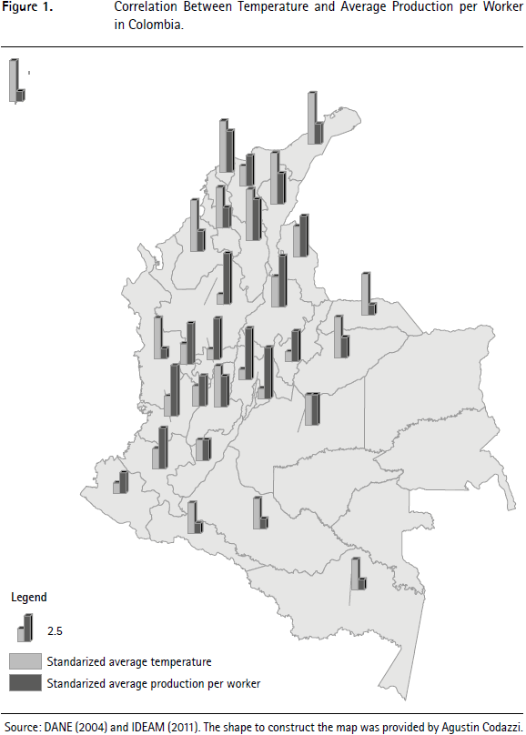
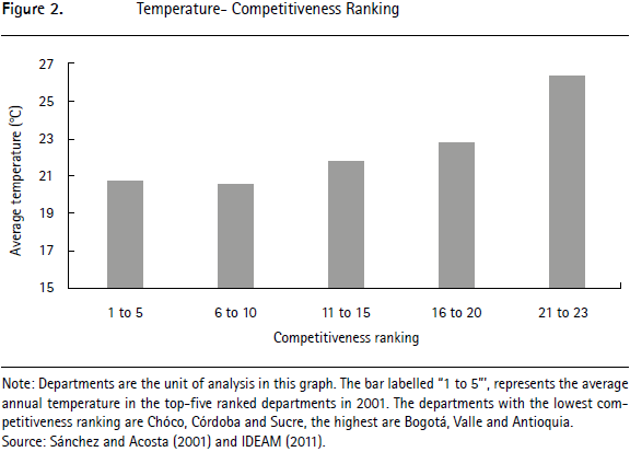
There is evidence that suggests a correlation between temperature and income in Colombia. This evidence is shown in Figure 1. In the map, one bar is worker output and the other is temperature. Most departments have one big bar together with a small one. Figure 2 illustrates a positive correlation between the competitiveness ranking⁶ and temperature (Sánchez & Acosta, 2001). This means that the departments that are ranked within the top five in Colombia (including Bogotá D. C., Valle, Antioquia) tend to have lower temperatures compared to Chocó, Córdoba and Sucre that are ranked last. Even if these are only correlations that do not represent causality, they suggest a strong effect.

The estimates report large, generally negative effects of higher temperatures on a worker's productivity. Changes in precipitation have relatively mild effects on national growth, but is still important to include them because they affect both temperature and income. This paper finds consistent results across a wide range of specifications, including a robustness check.

After this introductory section, the production function model will be presented, and the section will conclude with the level-growth theory. Section 2 describes the data sources, the methodology for constructing the indicators used in the empirical exercises and the descriptive statistics of the merged data set. Section 3 presents the empirical framework used to measure the effect of temperature on the output per worker, the presentation of the results and also an alternative model that is used as robustness check. Finally, conclusions are presented together with some policy suggestions.

I. Temperature in the Production Function: A Theoretical Model

This section analyses the channels through which temperature affects the current output per worker and the growth of output per worker over time in the manufacturing industry. In both cases, thermal stress having an impact on a workers' performance seems reasonable.⁷ In the long run, the creation of a working culture could be affected by the effect of thermal stress in the short run.⁸

Contemplating the impact of temperature on the growth of average output per worker in the long-run makes climate change relevant. If temperature shifts have an impact on current economic performance and economic growth, climate change will, in turn, affect these variables by affecting temperature patterns.

The future implications of climate change are very difficult to estimate and the empirical scope of this study is historical and short-term. Notwithstanding, this section explores a theory using which this long-term phenomenon could affect economic performance; however, it still takes into consideration uncertainties about the extent and nature of climate change. The analysis is based on four main effects that need to be controlled in order to make consistent long-term conclusions. First, it is possible that countries adapt to permanent changes in climate. Second, as climate change becomes a global issue, it may affect sea-levels, biodiversity and frequency of extreme climatic events that could simultaneously impact economic variables. Third, there is a big chance that mandatory mitigation actions will be implemented, and they may distort economic performance. Fourth, convergence forces may offset the impact of climate on the economy, especially within poor countries (Solow, 1956). The compounded effect of these four factors can turn the small effects found in this paper into long-term issues with major consequences.

The theoretical framework is a modification of the model presented in Dell et al. (2009) that develops a long-term mathematical relationship between temperature and average output per worker. The modification consists of using a specific production function in order to theoretically justify the empirical estimation of the missing parameter γ. It is important that in this case the analysis is only undertaken for the manufacturing industry with the purpose of isolating the effect that climate has on the output of capital.

The long-term effect of temperature on output per worker can be summarized into two broad categories⁹: adaptation and convergence. These have opposite effects given that convergence tends to increase the output per worker and adaptation tends to produce the opposite result.

It is important to clarify that the concept of convergence comes from the neoclassical theory and is based on the assumption that factors of production grow at the same rate in all countries; this has its roots in the decreasing marginal returns to scale of the factors of production. Additionally, the Colombian growth trend is upward sloping, and, hence, it can be said that the convergence level is above current levels. Therefore, the convergence effect will increase output per worker in the long-term, which is a natural inertia.

Moreover, the adaptation effect is directly related to temperature. The relationship is based on the fact that, in the long-run, areas must adapt to changes in geographic conditions such as climate. In the case of industries (the unit of analysis in this paper), the adaptation effect impacts the capital and labour sides of the production function. In terms of capital, there is an adaptation of technology and physical capital. More specifically, industrial establishments face costs caused by the variation of climate in the long-run. Hoverer, on the labour side of the production function, the adaptation occurs through migrations, fertility and mortality rates. People are forced to do things because of geographic conditions; in general, there are alterations on the industry's relative factor intensity.

The differential equation (1) is the starting point that summarizes the effect of temperature on output per worker¹⁰. It can be interpreted as the evolution of output per worker over time, and it depends on the adaptation and convergence effects.

where y is the income per capita, y. is the income per capita to which the regions converge, T_i is the temperature and _i is the average temperature of the municipalities where the industry i is present. The subscript i represents the industry and t the period. The coefficient γ captures the short-term effect of temperature, and ρ captures the degree of adaptation to the average temperature in the long-term. Finally, φ represents the convergence rate.

Integrating the differential equation (1) and taking expectations, the following is obtained,

Then, differentiating equation (2) with respect to temperature,

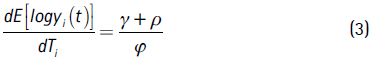
Equation (3) shows that the changes in output per worker, with respect to a change in average temperature, depends on the convergence parameter (φ), the effect of temperature in the short-term (γ) and the degree of adaptation to average temperatures in the long-term (ρ).

Dell et al. (2009) calculate 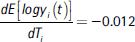in a within-country context. The convergence parameter, much analysed in the growth literature, is typically estimated in the cross-country context in the range 0.02< φ <0.1 (Barro & i Martin, 1995). The convergence rate is calculated between countries so, for the purpose of this paper, the upper bound will be used as the convergence within countries is higher (Caselli et al., 1996). The only two parameters left to calculate are ρ and γ. There is no estimation of the within country short-term growth coefficient in the literature; therefore, the empirical section of this paper is devoted to calculating it. The result for the Colombian manufacturing industry presented in Section 4 is γ = -0.003¹¹ (see Table 1). Due to the lack of information, Dell et al. (2009) use country level estimate: γ = -0.001. Finally, from equation (3) and, by undertaking a sensibility test, it is possible to calculate a range for the adaptation parameter 0.019< ρ <0.0029.

The rest of this section is used to explain how γ is calculated. This parameter is defined as the within country short-term growth coefficient. In order to estimate it, the methodology must disregard the long-term effects (adaptation and convergence) and focus on the short term in order to develop a hypothesis that is testable with the data available.

To begin, it is important to point out that recent empirical literature on economic growth estimates specifications based on variants of the Solow model in which the long-term growth rate of output per worker is determined by technical progress, which is taken to be exogenous. The most popular model used to evaluate this framework and to study the issue of convergence is derived from transition dynamics to the steady state growth path; it was first suggested by Mankiw, Romer and Weil (1992).

The model presented below is based on the theoretical framework by Bond, Leblebiciog and Schiantarelli (2009). For the specific scope of this study, a singlesector economy was chosen for the simplicity of the Y = AK type production function. The motivation for choosing this specific type of model is that the study focuses on the impact climate has on workers output. The manufacturing industry was chosen because climate will not affect the output of capital, which is the other factor that is taken into account in traditional production functions. In fact, the assumption here is that the other production factors will not be affected by the variance of the climate in a specific municipality between quarters. It is relevant to clarify this as the empirical methodology compares a municipality to itself through time. For instance, consider the following production function that incorporates temperature:

where Y is aggregate output, L measures workforce, A measures labour productivity and T measures weather. Equation (4) captures the relationship between weather and production.

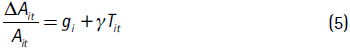
Equation (5) represents the growth of labour productivity that is affected by weather.

Now, dividing both sides of equation (4) by L_it, taking logs, differencing with respect to time and replacing equation (5) yields:

where g_it is the growth rate of output per worker (dependent variable) in the short-term. There is a direct link between equation (1) and (6). It is obvious that equation (6) ignores the long-term effects such as convergence and adaptation, but it includes the temperature lag in order to control for short-term lagged impacts of temperature on output per worker. The level effects of weather shocks on g_it, which come from equation (4), appear through β. The growth effects of weather shocks, which come from equation (5), appear through γ. Thus, equation (6) implies that it is not only current levels of average output per worker that are affected by temperature, but also the growth of the average output per worker. It also implies that temperatures from previous periods may have an impact. The aim of the empirical exercise is to estimate γ from a variant of regression (6) for the case of Colombia.

II. Data

The task of measuring the impact climate has on the average output per worker in the short-term(γ) is done by merging and analysing several datasets. The datasets that are described in this section complement each other in order to use the most precise and disaggregated information available. Some indices have had to be constructed in order to obtain the quarterly average output per worker, which, ultimately, is the dependent variable. Since the richness of the analysis lies in the comparison between hotter and colder periods, it is vital for the data to be quarterly. The variance of temperature and precipitation within years is larger than their variance between years, even in a country without seasons such as Colombia.

The challenge is to construct a dataset with the information available for Colombia that has quarterly climate variables for each municipality and production variables for each industry (ISIC).

The National Bureau of Statistics (DANE) has constructed the Annual Manufacturing Survey (AMS), which aims to obtain basic information from the Colombian industrial sector in order to characterize its structure and evolution. An unbalanced panel¹² records data for all industrial establishments with ten or more employed workers, or that had a production value of more than $130.5 million pesos in 2005¹³. Some of its variables are: number of employees, expenditure in wages and salaries, total value of production, total expenses, production costs, energy consumption, etc. The information is available for the industry in each municipality, it covers the period from 1993 to 2004, and has an annual frequency.

The Monthly Manufacturing Sample (MMS) constitutes another valuable source of information. It contains monthly data on the value of production, value of sales, size of the workforce, expenditure on wages and salaries, social benefits given to employees and average hours worked. To preserve anonymity, DANE publishes indices and variations. Using the Annual Manufacturing Survey (AMS) as reference, the MMS was designed to include 1344 randomly chosen establishments employing ten people or more. The resulting data is a representative sample of the manufacturing industry. It has been divided into 48 groups according to the third revision of the International Standard Industrial Classification adapted for Colombia (ISIC Rev. 3 A.C). The base year for this sample is 2001. From now on, all results will be presented in constant 2001 Colombian pesos.

For the climate variables, the information is obtained from the Institute of Hydrology, Meteorology and Environmental Studies (IDEAM for its Spanish acronym). This dataset is an unbalanced panel that contains monthly information for 772 municipalities in Colombia for the years 1931 to 2005. Some municipalities have more than one climatological station and therefore more than one observation. The variables available are maximum, median and minimum temperature, precipitation, humidity and solar radiation. The data before 1980 is incomplete but this will not matter as the merge will only take into account the data between 2001 and 2004 because of information constraints.

The main purpose of the following sub-sections is to explain the merge between the MMS and the AMS. This step is necessary because the empirical section uses a dataset on the municipal level (to be able to match the weather data) with quarterly coverage (to be able to exploit the intra-year variation of temperature). The AMS, has municipal disaggregation but is annual. On the other hand, the MMS is quarterly (at least the public version), but it is not disaggregated by municipality. The methodology used in this section can be viewed as a statistical matching technique, in which I observe subsamples of the same industrial establishments in both surveys and make some minor assumption to disaggregate the data to the level that I need (D'Orazio, Zio & Scanu, 2006). In summary, the market share by municipality is calculated from the AMS and is used to disaggregate the MMS.

The main assumption of this methodology is that the market share remains constant within a year (the variation across years is low so the assumption is reasonable). This is the main reason why the number of firms is used to calculate the market share. It is possible that production varies considerably within a year across municipalities; however, the number of companies in each industry is relatively structural and remains largely constant throughout quarters.

A. Market Share and Labour Share of each Municipality within an Industry

Since the quarterly data from the MMS is divided by ISIC but not by municipality, I used the information from the AMS to obtain quarterly data for each municipality. The indices used to do this are the market share and the labour share of each municipality within an industry in a specific year. These indices are calculated using the number of companies (total production is also used as a robustness check) and the work force.

where produc and labor are the number of firms and work force respectively. The subscripts i, m and t from now on correspond to industry, municipality and year. The top limit of the sum N_i depends on the number of municipalities in which the industry i is present. The market share and labour share will be useful to separate the MMS indices in municipalities.

B. Quarterly Output per Worker

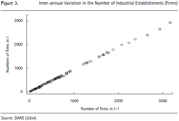
The MMS contains quarterly indices of production, employment and sales. The index is the value of the variable in a quarter divided by the value of that same variable in the first quarter of 2001 (2001q1: base period). As has been previously mentioned, these indices are not divided into municipalities. This means that from the MMS we have iproduc_iq (where q is quarter) and from the AMS mktshare_imt. The problem is symmetric for labour. By merging the two datasets and assuming that the market share is constant within years, it is possible to calculate the iproduc_imq. Again, the main assumption is that that the market and labour shares do not change within years. The fact that the market and labour shares do not change significantly between years suggests that the assumption is reasonable (see Figure 3). To convert these indices into the average output per worker, we used the following algebraic manipulation. By dividing both indices, we can obtain the following:

After some algebraic manipulation, the following was obtained:

This is the quarterly average output per worker that is used as a dependent variable in the empirical estimations. The growth rate of prodl_imq, g_prodl_imq is calculated with a standard methodology and will also be used as dependent variable.

C. Matching the Weather Data with Each Municipality

This paper calculates the municipal average temperature and precipitation based on data from the weather station that is closest to the largest populated area. The motivation to do so is in line with the issues identified in Auffenhammer, Hsiang, Schlenker and Sobel (2013). The size of each municipality means that there is a risk of measurement error for the explanatory variable. However, there are three reasons that explain why this is not a problem for the identification strategy. First and foremost, since the paper only studies the manufacturing industry, most of the establishments are located in the municipality's largest town (or the cabecera municipal). Luckily, these places also happen to have the majority of the weather stations. Using gridded or satellite data would contribute more noise than actual information; hence, I use the stations that are located in the largest populated areas of each municipality. Second, the potential measurement error is random and potentially very small, which generates a negligible attenuation bias of the estimator. Third, one of the main problems when using averages is that coverage is usually spotty (i.e. there are a lot of missing values or stations coming in and out of the sample). Since the data used in the paper is gathered on a quarterly basis, a missing value in a specific day or even week does not have a major impact on the accuracy of the explanatory variable.

Finally, it is important to highlight that the resulting panel does not contain establishment level data. Instead, it is aggregated on industry level. Therefore, the unit of analysis is the industry in each municipality of the country for the all quarters between 2001-2004.

D. Summary statistics

The summary statistics are presented in Table 2. The table summarizes the data used in the regressions, which cover the sixteen quarters between 2001 and 2004, for nineteen industries in 125 municipalities. The panel is set as the combination of the 633 different combinations of industries and municipalities (panel variable) for the sixteen quarters mentioned above (time variable).

The table divides variation into the following categories: overall, between and within. These categories arise because of the panel structure of the data. As the name suggests, the overall category summarizes all the 8,760 observations in the sample. The between variation is the variation between industries and municipalities. The within variation represents the variation that is exploited in the empirical strategy, which is the variation within the same municipality and industry and through quarters. The minimum and maximum numbers in the between and within categories are demeaned, which is why some numbers are negative.

The first variable shown in table 1 is the independent variable: prodl. As was mentioned in the data section, this variable represents the average output per worker in millions of pesos in the year 2001. The interpretation of the overall mean is that the average worker produces 15,87 million pesos in a quarter. The standard deviation is very large because it includes firms from all industries and all municipalities. There are very large and very small values for this variable; for example, for the Manufacture of general purpose machinery in Espinal, Tolima the value is very large because it refers to a capital intensive industry, which registered enormous production with only two workers. This variation is controlled by the industry-municipality fixed effect that makes sure outcomes between industries and municipalities are never compared. The within variation perfectly illustrates this point: the standard deviation is much lower as it is only compared within an industry-municipality group for the sixteen quarters. The empirical section also uses logarithms to control for potential outliers.

The second variable is the growth rate gprodl, which shows that the manufacturing industry has been growing at a moderate pace (0.5 %) over the quarters; this is roughly the same rate as the aggregate GDP.

The third and fourth variables summarize the weather in the 125 municipalities, which are for the most part the largest urban areas where the manufacturing industry is present. The main purpose of this table is to show that even though Colombia has almost indiscernible seasons, there is significant variance within years. The average temperature for the entire period of study is 21.68°C, with a standard deviation of 5.62, a minimum value of 4.17 in Villamaría, Caldas and a maximum value of 30.97 in Valledupar, Cesar. It is also important to note that the data recorded is an average for the whole day, not only the working hours. In terms of precipitation, the country average for all quarters is 116.9mm, with El Carmen de Atrato, Chocó presenting the highest levels of rainfall and four municipalities in La Guajira registering no rainfall during the period of study.

III. Estimation of the Effect of Temperature on the Average Output per Worker

In this section, the estimation models are described and the results are discussed. Furthermore, a robustness check is presented.

A. Empirical Framework

The empirical model of the study is based on Hsiang (2010) and borrows some concepts from Bogliacino and Pianta (2009) and Dell et al. (2009) that use a similar panel approach to this problem (Bogliacino & Pianta, 2009; Dell et al., 2009; Hsiang, 2010). It is a regression with industry-municipality and time fixed effects. The output per worker is explained as a function of its lags and the climate variables.

The objective of this study is to determine empirically if the mean output per worker in individual industries has any statistical dependence on intra-annual variations in the local temperature. Previous research used a cross-sectional approach in which patterns of production are correlated with the average state of the local atmosphere. A critique of this approach is that the average state of the atmosphere (a fixed parameter) may be correlated with other fixed parameters (for example, altitude), which may then directly affect patterns of production (Tol, 2009). This is the omitted-variables problem: without describing all fixed variables affecting an outcome, statistical inference on any single fixed variable may be biased (Greene, 2008).

Since it is almost impossible to control for all of these fixed variables, this study inserts industry-municipality and time fixed effects in order to only examine the effects related to dynamic variations. The average atmospheric states of any two municipalities are never compared here. Instead, the influence the atmosphere has on production is identified by looking at the response of production to perturbations in the atmospheric state around its mean value. This means that a municipality should only be compared to itself at different points in time when it is experiencing different atmospheric states. To avoid the omitted variable problem mentioned above, the precipitation is also included in the regression; this, together with temperature constitute the atmospheric state (Auffenhammer et al., 2013). Some argue that cyclones should also be included as they are correlated to temperature and production (Hsiang, 2010). In the case of Colombia, cyclones are not a major problem and are mostly isolated atmospheric phenomena that are not relevant for the study of this specific country.

Given the variables calculated in the previous section, the following two regressions can be run with fixed effect of industry-municipality, lags, time fixed effect and environmental variables.

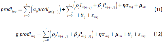
The difference between regression (11) and (12) is the dependent variable. In the first regression, it is the level of output per worker and in the second it is the growth rate. For both regressions μ_im is the industry-municipality fixed effect, θ_q is the time fixed effect, σ_mq is the temperature variance, P_m(q-j) is the precipitation and T_m(q-j) is the temperature (all variables in equation (11) are in logarithms). The parameter of interest is, therefore, ρ_j, which accompanies the temperature indicator. Since the survey is a panel, the regression is run where i is the industry, m the municipality and q is the quarter. The industry municipality fixed effect is very important because it captures all the statical differences in levels of production between industries and municipalities. Finally, the time fixed effect captures all changes in average output per worker that vary smoothly over time for all industries and municipalities equally. To calculate J, the Durbin's h-test is performed to check for serial correlation. The lags are included as long as they are statistically significant. For L, the literature states that only one lag is necessary.

The empirical strategy estimates (11) and (12). The following null hypotheses are tested in order to assess if temperature has no effect on growth:

Hypothesis (13) is relevant because if it is not rejected, it would mean that there is an absence of both level and growth effects within the entire manufacturing industry. If we reject the null hypothesis, the parameter ρ_j will be our estimator of the coefficient (γ), which is needed to complete the long-term model. Following the conventions in the distributed-lag literature (Greene, 2008), the growth null hypotheses is stated for the accumulated effect of temperature:

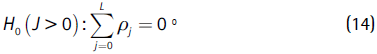
Null hypotheses (13) and (14) are tested for both regressions to explore the sign and magnitude of the parameter of interest γ. It summarizes the evidence of an effect of temperature on the growth of output per worker in the short-term.

1. Non-linear Effects of Temperature

Ergonomic studies state that the effect of temperature on productivity is nonlinear because in high-temperature places the effect is greater: "If the economic response to temperature is non-linear in agreement with ergonomic studies, temperature changes during the hottest season should have a greater economic impact than temperature changes in other seasons" (Pilcher et al., 2002). Figure 5 illustrates the mean percentage difference in performance between the neutral temperature groups and five temperature subcategories defined by the author.

Our interpretation is that performance is not altered when the mean temperature is in the Hot1 subcategory. When the temperature is below that level, performance is lowered because of the cool environment, and when it is beyond that point, performance is lowered because of the hot environment. From the total of 125 municipalities in the sample, 67 have higher temperatures than Hot1 and 24 have lower, leaving 34 in the temperature comfort zone.

Some interesting conclusions emerge when the ergonomics findings are applied to the Colombian case. The minimum average temperature of the areas where the productive activities take place is very close to the bottom frontier of Hot1, where performance is not altered. In fact, only four departments show temperatures below that subcategory: Nariño, Boyacá, Cundinamarca and Caldas. The purpose of this explanation is to show that Colombia will not be positively affected by an increase in its average temperature driven by climate change; on a department and municipality level the evidence is clear. This conclusion is due to the fact that most of the productive activity in Colombia is undertaken where the temperature is in subcategories Hot1 and Hot2. The mean 21.68°C is also evidence of this. The ergonomics findings in this area are relevant because they suggest the existence of non-linearity on the impact of climate change.

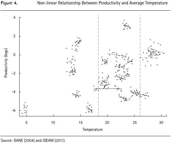
The evidence in Figure 4 is in line with Pilcher et al. (2002) and shows possible non-linearity in the Colombian data. It is a graphic representation of the correlation between temperature and average output per worker for Manufacture of apparel; preparation and dyeing of fur (this specific industry was chosen from all industries for illustrative purposes only). The figure can be interpreted as a rough graphical representation of equation (11) (without the fixed effects or controls). Each dot represents the output per worker for a specific municipality for a specific quarter. The presence of clusters is expected as temperature and output per worker are highly correlated over time in specific municipalities; for this reason, the industry-municipality fixed effect is so important and, standard errors must be clustered and robust to control for heteroskedasticity and autocorrelation. The coloured lines are regression lines for each municipality, and the vertical dashed lines show the Hot1 thresholds (where productivity is optimal according to ergonomics findings). It is interesting to see how most coloured lines to the left of the threshold have a positive slope. Those within the Hot1 threshold show no clear trend (perhaps negative), while those to the right of the threshold show a clear negative trend. This is suggestive evidence for the presence of non-linearity.

In this paper, we develop one additional strategy to provide some evidence of the non-linear effects. The approach is to break the sample into the temperature categories identified in the lab experiments, expecting larger negative effects in the groups that have the highest average temperatures.

It is important to highlight that these methodologies only suggest the presence of non-linearity. However, further research is necessary, and, in this respect, the data used in this paper faces some challenges. It is difficult to capture non-linearity with this data because there is not a large enough variation in temperature within municipalities. Since the empirical strategy only compares the same industrymunicipality over time, the range of temperatures within these groups is never wide enough to capture proper non-linearity. According to (Pilcher et al., 2002), we would need to see municipalities that report quarterly variation ranging from at least Cold1 (10.81-18.28) to Hot2 (26.63-32.17). The within standard deviation in the dataset is 0.65 degrees, and the maximum is 5 degrees, from 17 to 22 in Pereira, which is too small for this type of analysis.

B. Results

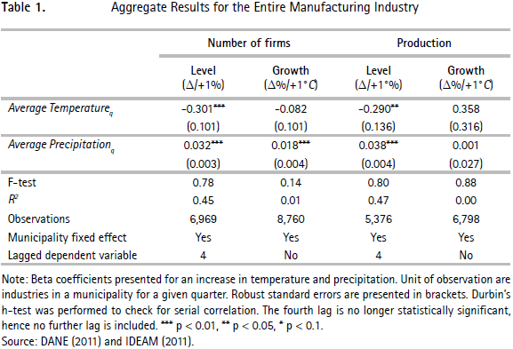
In this subsection, the results for both level regressions in equation (11)¹⁴ and growth regressions in equation (12)¹⁵ are reported and discussed (see Table 1). The first part of the section contains the results from the main regressions; the null hypotheses mentioned above are then tested with this data, and the parameter γ is calculated. The results of the empirical strategy designed to assess the non-linear effect hypothesis are presented at the end of this subsection (see Figures 4 and 3). The tables in the Tables and Figures section contain the complete results of the regressions. It is important to highlight that the null hypothesis (13) is directly tested with the resulting coefficients, and the null hypothesis (14) is tested with an F-test.

The first hypothesis that will be tested states that temperature does not affect average output per worker, either through level effects or growth effects (equation 13) in the entire manufacturing industry. As was previously mentioned, this hypothesis is tested for the aggregate regressions. Table 1 presents the results that show that when the estimation is made on an aggregate level, there is a negative statistically significant relationship between temperature fluctuations and the level of output per worker (-0.3 % / +1 %); there is also a negative but statistically insignificant relationship between temperature fluctuations and the growth of output per worker (-8.2 % / +1°C). The results hold for an alternative definition of the dependent variables. In columns 1 and 2 of Table 1, the dependent variable was calculated using the market share defined by the number of firms, while columns 3 and 4 use production. The sign and magnitude of the effects are similar in both cases. However, the F-test is very low, which does not allow the null hypothesis (14) to be rejected. The fact that the level is significant and the growth insignificant is expected because the time horizon of the study is not long enough to capture significant changes.

An important result that has been presented in this paper is the fact that the precipitation coefficients for all cases presented an opposite sign and smaller magnitude compared to temperature. This finding supports the hypothesis that climate alters the labour supply by shifting the opportunity cost of work over leisure. However, this hypothesis is not directly tested in this paper.

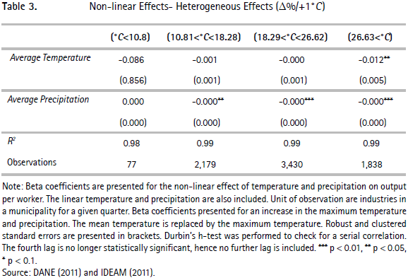
Figure 5 illustrates the non-linear effects of productivity as measured in the lab (Pilcher et al., 2002). However, measuring this type of non-linearity with field data is more challenging. Table 3 and Figure 4 present the results of the methodologies developed to assess the non-linearity of the effect of temperature on average output per worker. The industry regressions are run to check if deviations from the mean temperature in normally hot and cold municipalities have similar effects.

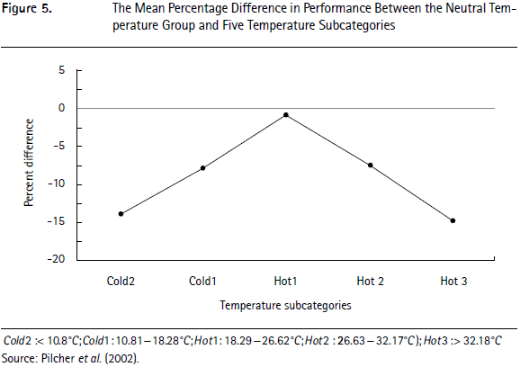
Table 3 shows that the negative coefficient is only observed in the Hot2 category: a temperature higher than 26.63°C. The coefficients in all remaining categories are not statistically significant. This is in line with the original lab results, which suggest that the impact is indeed larger in this context and provide some evidence of the above mentioned non-linearity.

C. Robustness Analysis

An additional empirical exercise confirms the robustness of the negative effects of temperature on the main variables of interest. This section contains an alternative specification as a robustness check.

1. Alternative Sample and Data Sources: Regression with Geo-referenced Temperature Data and CEDE Yearly Municipal Panel

This section contains the same empirical framework applied to a data set with different characteristics. This data set is a panel that was constructed by the Center of Economic Development Studies (CEDE) between 1993 and 2010 on a yearly basis. It contains data from the presidency, the National Planning Department and DANE.

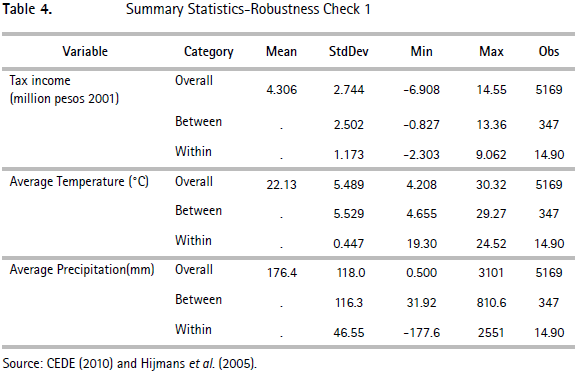
Using municipal level data for Colombia, this section shows the relationship between Geo coded climate variables (obtained from Worldclim (Hijmans, Cameron, Parra, Jones & Jarvis, 2005)) (mean temperature, mean precipitation levels and other climatic variables) and income. Since there is no data for income on a municipal level in Colombia, the independent variable is the proxy tributary income of industry and commerce. This makes sense since the taxes that firms have to pay are linearly related to the value added they produce. In turn, these variables are divided by the total workforce of the municipality to obtain the per-worker level, and the logarithm is then calculated in order to make the regression in levels. The summary statistics can be found in Table 4. The average temperature is similar to the one measured with the weather station data. In the case of precipitation, the calculations are substantially different. In both cases, the within variability is enough to allow for the application of the fixed effects methodology. The mean tax income per worker is four million pesos for all industrial establishments.

The inclusion of this robustness check responds to the pitfalls usually encountered in economic studies that use weather data (Auffenhammer et al., 2013). Calculating the average of a set of weather stations (such as in the case of this study), as well as the fact that some stations have intermittent coverage, may introduce measurement error. As was explained in the data section, this is not the case because most manufacturing establishments are located in the largest populated areas of the municipality, which is where most weather stations are located. Additionally, the use of quarterly data diminishes the risk of having biased results because a few days' worth of data are missing. However, using gridded weather data from Worldclim removes any suspicion of measurement error.

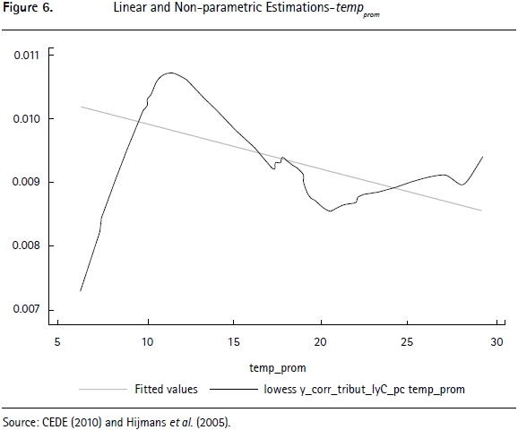
The results of this subsection support the previously reported results. As shown in Figure 6, the results that come from this data are in line with the general empirical results. Both linear and non-parametric estimations show a negative correlation between the tributary income of industry and commerce and the mean temperature. Additionally, the non-parametric estimation illustrates a non-linear effect that is in line with the lab results from Pilcher et al. (2002).

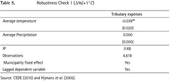
The empirical framework explained above is also applied to this data set, and the results are available in Table 5. Similarly to the other results, there is a negative statistically significant coefficient of mean temperature on output per worker. Since the weather data in this case comes from a gridded approximation, the accuracy is inferior to that from the actual weather station data.

Conclusions

This study uncovered evidence relating to the effect of temperature and precipitation on the average output per worker. It builds on previous literature that argues that in fact worker's productivity is a channel through which climate and climate change affect economic performance. The study is relevant in the economic growth theory complementing Hall and Jones' (1999) theory by saying that social infrastructure should have a healthy environment as one of its components, in this case through sustained moderate temperatures. Calculating the short run effect of temperature on growth within the country is a key component of the long-run model that was previously unknown in the case of Colombia. In the long-run, climate change will increase average temperature, and according to the results of this paper, will in turn affect output per worker.

In terms of public policy, the study presents empirical evidence for an alternative channel through which climate change will impact sectors of the manufacturing industry. It presents ergonomics as new area of interest for the Low Carbon Development Strategy and the National Adaptation Plan. The quantification of this impact constitutes an incentive for the industry to mitigate carbon emissions in order to maximize the benefits in the long-term. Finally, these results could help environmental agencies and researchers to more accurately calculate the costs of climate change in the long-run. They could also provide valuable inputs for international and sectoral negotiations.

This paper does not constitute experimental evidence, and, therefore, causality should be inferred carefully. Omitted variables such as unemployment or violence are potential threats to the identification strategy. Experimental data or the exploitation of a natural experiment should be carried out to generate causal evidence.

The methodology could be used with more disaggregated data in order to obtain more accurate and robust results. It is likely that since the unit of analysis is a whole industry, some detailed effects have been overlooked. The same methodology will surely be more useful with industrial establishments as the unit of analysis. Further work could also be carried out, that is in fact more robust and statistically significant, to analyse the effect of precipitation. It would also be interesting to repeat this exercise with municipal quarterly data directly taken from the MMS, instead of making assumptions in order to merge the AMS with the MMS. Regarding the climatic variables, it would be helpful to use temperature for working hours only. It would also be interesting to see a dataset that can properly capture the non-linearities, and not only though approximations.

_____________________________
Foot notes
² Social infrastructure is defined as "the institutions and government policies that determine the economic environment within which individuals accumulate skills, and firms accumulate capital and produce output"' (Hall & Jones, 1999).
³ Ergonomics studies the design and arrangement of things people use in order to make their interaction safer and more efficient.
⁴ The ergonomics of thermal stress on humans has been well studied, and there is a lot of literature on this topic. Laboratory experiments show that when the temperature is higher than 26.62°C WGBT and lower than 18.29°C productivity drops. The WGBT is a composite temperature used to estimate the effect that temperature, humidity, wind speed and solar radiation has on humans. (U.S. Army Technical Bulletin Medical 507/Air Force Pamphlet 48-152) (Pilcher, Nadler & Bush, 2002). This is evidence of the non-linearity that is mentioned above.
⁵ The motivation for choosing this specific type of model is that the study focuses on the impact climate has on workers output. The manufacturing industry was chosen because the climate will not affect the output of capital, which is the other factor that is taken into account in traditional production functions.
⁶ The competitiveness ranking is based on an index that is calculated to measure all the departments in Colombia's level of economic performance.
⁷ "Three of six non-agricultural industries suffer large and robust reductions in annual output that are dominated by temperatures experienced during the hottest season and are non-linear in temperatures during that season. The magnitude, structure and coherence of these responses support the hypothesis that the underlying mechanism is a reduction in the productivity of human labor when workers are exposed to thermal stress" (Hsiang, 2010).
⁸ The Pygmalion effect refers to the phenomenon that the higher the expectation placed upon a person the better that person performs (Rosenthal & Jacobson, 1992); Temperature altering the Circadian rhythm (in biology, circadian rhythms are oscillations of biological variables at regular intervals of time); and implications on the allocation of time. Temperature affects the opportunity cost of working over leisure. Following this logic, it will also affect labour supply (Graff & Neidell, 2014).
⁹ Mitigation is another category that is neither related to adaptation or convergence. Universidad de los Andes is now calculating the abatement cost curves (net present value of mitigating climate change) under the Low Carbon Development Strategy framework. Once these values are available, it would be interesting to redesign this model in order to calculate the impact such measures have on the long-term growth of output per worker. The way the adaptation parameter is calculated ensures that impacts on other environmental variables such as biodiversity are accounted for.
¹⁰ This equation is an application of the model derived in Dell et al. (2009).
¹¹ The result is the average country short-term coefficient for the Colombian manufacturing industry.
¹² All regressions are calculated using the balanced panel. The panel is lightly unbalanced (the biggest difference in observations between years is never more that 1%. Industrial establishments coming in and out of business, as well as passing the sampling threshold, are the main reasons for the panel being unbalanced). Therefore, the data is not censored.
¹³ This assumption had to be made due the National Bureau of Statistics' (DANE) budget constraints.
¹⁴ All variables are in logarithms and therefore results are in elasticities.
¹⁵ All variables are in original units. These variables were left in original units because the logarithm can only be taken when all values are positive.

References

1. Acemoglu, D., Johnson, S., & Robinson, J. (2002). Reversal of fortune: Geography and institutions in making of modern world income distribution. The Quarterly Journal of Economics, 117(4), 1231-1294.         [ Links ]

2. Arrow, K. (2004). Are we consuming too much? Journal of Economic Perspectives, 18(3), 147-172.         [ Links ]

3. Auffenhammer, M., Hsiang, S., Schlenker, W., & Sobel, A. (2013). Using weather data and climate model output in economic analyses of climate change. Review of Environmental Economics and Policy, 7(2),181-198.         [ Links ]

4. Barro, R., & i Martin, X. S. (1995.). Economic Growth. London: McGraw-Hill.         [ Links ]

5. Bogliacino, F., & Pianta, M. (2009). The impact of innovation on labour productivity growth in European industries: Does it depend on firms' competitiveness strategies? (Working Paper). ITPS.         [ Links ]

6. Bond, S., Leblebiciog, A., & Schiantarelli, F. (2009). Capital accumulation and growth: A new look at the empirical evidence. Journal of Applied Econometrics, 25(7), 1073-1099.         [ Links ]

7. Burke, M., Hsiang, S., & Miguel, E. (2015). Climate and conflict. Annual Review of Economics, 7(1), 577-617.         [ Links ]

8. Cadena, A., Rosales, R., Salazar, M., Rojas, A., Delgado, R., & Espinosa, M. (2012). MAPS: Colombia case study (Working Paper). MAPS.         [ Links ]

9. Caselli, F., Esquivel, G., & Lefort, F. (1996). Reopening the convergence debate: A new look at cross-country growth empirics. Journal of Economic Growth, 1(3), 363-389.         [ Links ]

10. CEDE (1993-2010). Panel Municipal del CEDE-Universidad de los Andes. (Working Paper). CEDE.         [ Links ]

11. CONPES (2011). 3700-Estrategia institutcional para la articulación de políticas y acciones en materia de cambio climático en Colombia. Technical report, DNP. http://oab2.ambientebogota.gov.co/es/documentacion-e-investigaciones/resultado-busqueda/conpes-3700-estrategia-institucional-para-la-articulacion-de-poli-ticas-yacciones-en-materia-de-cambio-climatico-en.         [ Links ]

12. D'Orazio, M., Di Zio, M., & Scanu, M. (2006). Statistical Matching. London: Wiley.         [ Links ]

13. Daly, H. (1996). Beyond Growth: The Economics of Sustainable Development. Boston: Beacon.         [ Links ]

14. DANE (1993-2004). Annual Manufacturing Industry. Technical Report. Departamento Nacional de Estadística. https://www.dane.gov.co/files/investigaciones/boletines/eam/boletin_eam_2015.pdf.         [ Links ]

15. DANE (2001-2011). Monthly Manufacturing Sample. Technical Report. Departamento Nacional de Estadistica. https://www.dane.gov.co/index.php/comunicados-y-boletines/industria/mmm.         [ Links ]

16. Dell, M., Jones, B., & Olken, B. (2012). Climate change and economic growth: Evidence from the last half century. American Economic Journal: Macroeconomics, 4(3), 66-95.         [ Links ]

17. Dell, M., Jones, B., & Olken, B. (2009). Temperature and income: Reconciling new cross-sectional and panel estimates. American Economic Review: Papers & Proceedings, 4(3), 66-95.         [ Links ]

18. Dell, M., Jones, B., & Olken, B. (2013). What do we learn from the weather? The new climate-economy literature. Journal of Economic Literature, 52(3), 740-798.         [ Links ]

19. D'Orazio, M., Zio, M. D., & Scanu, M. (2006). Statistical matching. London: Wiley.         [ Links ]

20. Gallup, J. L., Sachs, J. D., & Mellinger, A. (1999). Geography and economic development (Working Paper). CID.         [ Links ]

21. Graff, J., Hsiang, S., & Neidell, M. (2015). Temperature and human capital in the short- and long-run. Cambridge: NBER.         [ Links ]

22. Graff, J., & Neidell, M. (2013). Environment, health and human capital. Journal of Economic Literature, 51(3), 689-730.         [ Links ]

23. Graff, J., & Neidell, M. (2014). Temperature and the allocation of time: Implications for climate change. Journal of Labor Economics, 32(1), 1-26.         [ Links ]

24. Greene, W. (2008). Econometric analysis. Cambridge: Pearson.         [ Links ]

25. Hall, R. E., & Jones, C. I. (1999). Why do some countries produce so much more output per worker than others?. The Quarterly Journal of Economics, 114(1), 83-116.         [ Links ]

26. Hijmans, R., Cameron, S., Parra, L., Jones, P., & Jarvis, A. (2005). Very high resolution interpolated climate surfaces for global land areas. International Journal of Climatology, 25(15), 1965-1978.         [ Links ]

27. Hsiang, S. (2010). Temperatures and cyclones strongly associated with economic production in the Caribbean and Central America. Proceedings of the National Academy of sciences, 107(35), 15367-15372.         [ Links ]

28. IDEAM. (2011). Temperature and precipitation data. IDEAM. https://www.datos.gov.co/.         [ Links ]

29. Mankiw, G., Romer, D., & Weil, D. N. (1992). A contribution to the empirics of economic growth. The Quarterly Journal of Economics, 107(2), 407-437.         [ Links ]

30. Nordhaus, W. (2006). Geography and macroeconomics: New data and new findings. Proceedings of the National Academy of Sciences of the United States of America, 103(10), 3510-3517.         [ Links ]

31. Pilcher, J., Nadler, E., & Bush, C. (2002). Effects of hot and cold temperature exposure on performance: A meta-analytic review. Ergonomics, 45(10), 682-698.         [ Links ]

32. Ramsey, F. (1928). A mathematical theory of saving. The Economic Journal, 38(152), 543-559.         [ Links ]

33. Rodrik, D., Subramanian, A., & Trebbi, F. (2002). Institutions rule: The primacy of institutions over geography and integration in economic development. Journal of Economic Growth, 9(2), 131-165.         [ Links ]

34. Rosenthal, R., & Jacobson, L. (1992). Pygmalion in the classroom: Teacher expectation and pupils' intellectual development. London: Crown House Publishing Limited.         [ Links ]

35. Sachs, J. (2003). Institution don't rule: Direct effects of geography on per capita income (Working Paper). NBER.         [ Links ]

36. Sachs, J. D., & Warner, A. M. (1997). Sources of slow growth in African economies. Journal of African Economies, 6(3), 335-376.         [ Links ]

37. Sánchez, F., & Acosta, P. (2001). Proyecto indicadores de competitividad: Colombia. Proyecto Andino de Competitividad. Documento de trabajo. Reporte técnico. CID, Harvard University.         [ Links ]

38. Smith, A. (1776). An inquiry into the nature and causes of the wealth of nations. London: W. Strahan and T. Cadell.         [ Links ]

39. Solow, R. (1956). A contribution to the theory of economic growth. Quaterly Journal of Economics, 70(1), 65-94.         [ Links ]

40. Somanathan, E., Somanathan, R., Sudardhan, A., & Tewari, M. (2015). The impact of temperature on productivity and labor supply: Evidence from Indian manufacturing (Working Paper). CDE.         [ Links ]

41. Stern, N. (2006). Stern review: The economics of climate change. Technical report. Cambridge: Cambridge University Press.         [ Links ]

42. Tol, R. (2009). The economic effects of climate change. The Journal of Economic Perspectives, 23(2), 29-51.         [ Links ]