English (pdf)
 Article in xml format
 Article references
 Send this article by e-mail
 Cited by SciELO
  Cited by Google
  Similars in
SciELO
Similars in
SciELO  Similars in Google
 Permalink
The purpose of this study is to project eligibility and replacement rates for the Uruguayan social security system in its two pillars: mandatory individual saving accounts (defined-contribution) and the pay-as-you-go system (defined-benefit), which expresses them as a ratio of the last salary and the average working-life earnings. We aim to analyze both the coverage of the system and its ability to smooth consumption over its life cycle. Bucheli, Ferreira-Coimbra, Forteza & Rossi (2006) and Bucheli, Forteza, & Rossi (2010) estimate eligibility prior to the 2008 law (18395) that loosened access requirements to contributory pensions. This study updates projections for the percentage of individuals expected to become eligible for contributive pensions and most importantly, for the first time, estimates replacement rates for Uruguay using individual data from social security records. Studies that project pension replacement rates using administrative data are extremely scarce in the international literature. Using individual data is relevant because it allows us to analyze distributive implications and is of particular importance in countries with non-negligible levels of informality as most countries in Latin America.
Our data consists of a random sample of 14,207 contributors to the Banco de Previsión Social (Uruguay’s major social security agency) who in January 2017 were between 40 and 60 years old. Based on this sample, we estimate the probability of them contributing each month until they reach retirement age. We then model individual earnings based on personal characteristics and macroeconomic variables. We also project the accumulated fund in the mandatory individual savings account (FAP for its Spanish acronym). The high quality of the data used enables us to analyze heterogeneity among the cohort under study.
We compute gross replacement rates that result from considering both the defined benefit and the individual savings pillar as a whole (which we name joint replacement rate) and also analyze the replacement rate yielded by each pillar separately and simulate how different macroeconomic scenarios affect our results. We analyze the correlation of the resulting rates in terms of gender, age cohort, average density of contributions, income quintiles, and sector of activity. Furthermore, we examine how the rate of return of the pensions funds’ investments and management fees affect the final amount accumulated in the individual savings account and, subsequently, the annuity. Finally, for those individuals who have a high contribution density, we analyze the impact of postponing the decision to retire until age 65.
The paper is organized as follows: the next section describes the Uruguayan pension system. Section II reviews the related literature. Sections III and IV describe the sources of information and methodology used. Section V presents the results while section VI concludes.
I. The Uruguayan pension system
In 1996, the Uruguayan pension system administered by Banco de Prevision Social (BPS) was transformed into a “Mixed System” (Law 16713) with two pillars: a pay-as-you-go (PAYG) or defined benefit scheme and an individual savings accounts or defined contribution scheme. The system became compulsory for those under 40 as of April 1, 1996. A monthly earnings threshold separates the two pillars. Individuals with monthly wages lower than $5,000 (Uruguayan pesos in May 1995, approximately USD 1,700 in 2017) are served by the PAYG unless they explicitly choose to participate in the individual savings scheme. They can choose to assign 50% of their monthly contributions to the individual savings account (Article 8 Law 16,713). If they do, BPS grants a bonus and increases the individuals’ contributions to a defined benefit scheme by 50%. Earnings between $5,000 and $15,000 (Uruguayan pesos in May 1995) must contribute to the individual account; it is optional to do so for earnings above this amount.
Within the PAYG pillar, a minimum of 30 years’ contributions is required in order to be eligible (the minimum was set at 35 in 1995 and then reduced by Law 18,395 in 2008). Required years of contribution decrease if individuals retire at older ages (minimum of 15 years after 70). Women benefit from one year’s contribution per child (maximum of five years). The benefit not only improves eligibility conditions but also increases the replacement rate of the defined benefit scheme.
In the PAYG pillar, the earnings considered to calculate the pension are the average wage earned in the last 10 years. Depending on what is more beneficial for the worker, the average wage earned in the best twenty years (increased by 5%) may also be used. The rate applied is 45% and there is an additional 1% for every extra year’s contribution between 30 and 35. For thirty-six years of contributions onwards, every additional year worked adds 0.5% to the rate (there is a maximum of 2.5%). Moreover, for each year that the person postpones retirement after the age of 60 (whether s/he continues working or not) the replacement rate increases by two pecentage points. Therefore if an individual reaches age 60 with 30 years’ contributions and decides to continue working until 61, 48% will be used to calculate their pension.
As for the individual savings pillar, Law 16,713 created AFAPs that administer the savings fund (Fondo de Ahorro Previsional) that consists of the mandatory and voluntary workers´ contributions and its returns. AFAPs charge an administration fee and deduct an insurance premium (“Prima de Seguro Colectivo”) that covers the risks of disability and mortality during working life. The annuity depends on the final accumulated fund in the individual account, sex, and age at the time of retirement (which reflect the individuals´ life expectancy) and the probability of having a member of the family who can claim the pension as well as a technical interest rate. Individuals can cash their annuity when they retire from the PAYG system or at a minimum of 65.
II. Related literature
To the best of our knowledge, only one study from Chile projects pension replacement rates using administrative data. Berstein, Larrain and Pino, (2006) estimate the probability of future contributions using a probit model with random effects and an earnings model that includes individual characteristics and variables related to the macroeconomic context. Replacement rates are estimated at 121% of the average salary during the entire working life and 44% of the last salary. Paredes and Díaz Fuchs (2013), in turn, calculate replacement rates for Chile using the administrative data of individuals who had already retired in 2012. They estimate an average replacement rate for the old age pension (with at least 10 years’ contributions) of 76%. They additionally highlight the substantial differences due to gender and contribution densities.
OECD (2013) simulates replacement rates assuming individuals contribute to social security for 40 years earning the average wage in their respective country. For OECD member countries, the average gross replacement rate is estimated at 54%. Durán Valverde and Pena (2011) project replacement rates from the individual savings account systems of different Latin American countries using information from household surveys. In the case of Uruguay, they estimate replacement rates of 43% and 44% for men and wo-men, respectively, relative to the last wage and 39% and 38% for men and women relative to the average income of the last 20 years they worked. Forteza and Ourens (2012) analyze the characteristics of several Latin American pension programs evaluating their impact on income inequality, insurance, and incentives to work. They simulate lifetime contributions and benefits and conclude that most programs are progressive while implicit rates of return exhibit marked discontinuities in the length of service, which they attribute to vesting period conditions. A recent study by Altamirano, Berstein, Bosch, García- Huitrón and Oliveri, (2018) analyzes pension systems across Latin America and the Caribbean and consider hypothetical individuals with a perfect contribution record in the baseline scenario. For Uruguay, the estimate for the average replacement rate is 72% in the baseline scenario.
In contrast to the lack of studies that project replacement rates and eligibility while using individual administrative records, there is a greater abundance of literature that forecasts pension eligibility in Uruguay. Bucheli et al., (2010) estimate the proportion of workers who would gain access to a pension at the normal retirement age by using a random sample of work history records for individuals between 18 and 70 who contributed for at least one month between April 1996 and December 2004. They use survival analysis to model transitions between contributing and not contributing and then apply the estimated transition rates to project worker trajectories using Monte Carlo simulations. Their main findings suggest that, as workers spend more time in any of the two states (contributing or not contributing), their chances of remaining in the same state increases. They also find that young workers are more dynamic and have a higher probability of leaving either of both states. They project that only 41.3% of workers will have accumulated 30 years’ contributions at age 60. Also, they find very significant differences between income quintiles. It should be noted this study was carried out prior to the 2008 reform that relaxed pension eligibility requirements.
Forteza and Sanroman (2015) estimate a structural life-cycle model for retirement behavior using work history records. They find that individuals, especially women, prefer not to postpone retirement. They also find that retirement decisions are not particularly responsive to changes in retirement modification rules. More recently, Lavalleja, Rossi and Tenenbaum (2018) have studied the impact of the latest legal modification in pension requirements that was passed in 2008 using administrative records. Following Bucheli et al. (2006), they divide the sample into groups that consider sex, income level, and contribution sector and estimate the probability of contributing by group (conditional on the previous month’s contribution status). Subsequently, they simulate each group’s contribution history by using Markov chains. They conclude that for the minimum age of retirement (60), 38% of workers would be eligible for retirement under the current legislation compared to 11% under the 1996 regime (Law 16,713): a scenario in which the minimum years’ contributions had not been reduced from 35 to 30 and there was no bonus year per child for women.
Regarding other Regarding other estimates of pensions adequacy in Uruguay, Forteza and Rossi (2016) simulate theoretical pensions and replacement rates for those in their 50 in 2016 and compare them with those who retired from the PAYG system under the conditions prior to the 1996 reform. They conclude that some individuals in their 50 (mainly high-income) would have received a higher pension under the system prior to the reform. Alvarez, Silva, Forteza and Rossi (2010) focus on retirement incentives by comparing the PAYG system prior to the 1996 reform with the multi-pillar system. Using simulations for hypothetical individuals, they conclude that the 1996 reform improved the incentives to postpone retirement, but the incentives are still low compared to developed countries.
III. Data
This study uses a random sample of 14,207 workers´ administrative records for individuals aged between 40 - 60 years old as of January 2017 who contributed at least once as a dependent worker between 1996 and 2015. Using the Longitudinal Survey of Social Protection (2015), we estimate that the sample analyzed is representative of 73% of the age bracket (with the remaining 20% never contributing to social security and 7% contributing to other pension systems). The rest of the cohort either never made contributions to social security or made contributions to other schemes such as military, police, or professional ones. We concentrate on this age cohort because, given the policy debate that took place in 2016 – 2017, we were interested in comparing the fate of those in their 50, which was the first cohort about to retire from the multi-pillar system, with those 10 years younger. It should also be noted that no administrative records exist prior to 1996. The following table presents the descriptive statistics of the variables included in the database.
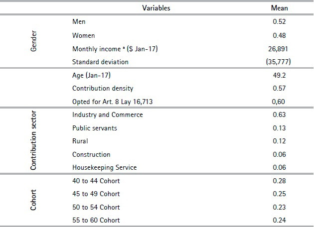
Table 1. Descriptive statistics (Cont.)
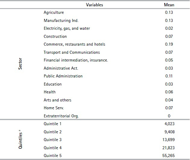
Source: Authors’ own calculations based on social security records. a) Income for 1996 - 2015 at January 2017 prices in Uruguayan pesos.
Figure 1 shows the distribution of the average contribution density for the employment history sample over the observed period (1996-2015). We observe a significant disparity in individuals’ contribution density. In the lower distribution tail, 31.6% of men and 26.9% of women contributed up to 30% in the 1996-2015 period, which is equivalent to a maximum of six years’ contributions of the 20 years considered. Moreover, approximately 25% persistently contributed (100%) during the period. It is also important to note that slightly less than 10% of the sample shows a contribution density of less than or equal to 5%, which means that they contributed to social security for at most 12 months between 1996 - 2015. This polarization in terms of contribution density highlights the importance of analyzing eligibility and replacement rates for the different segments of the distribution. The percentage of workers who did not contribute to the savings accounts pillar is estimated to be 32%. Indeed, even if approximately 75% of the workers are situated in the first income bracket, where contributions to the savings account are not compulsory, 60% of the sample opted for Article 8 of Law 16713, which enables voluntary contributions to the individual savings pillar.
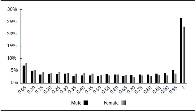
Source: Authors´ own computations derived from social security data.
Figure 1. Distribution of the observed contribution density by gender (1996-2015)We define contribution density as the relationship between the number of periods contributed by the employee to the social security system and potential contributions during his or her working life.
IV. Methodology
A. Contribution density and years of contributions
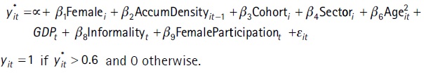
To project the contribution density, we model the probability of making monthly contributions to the social security system from 1996 onwards using a probit model with random effects including both individual characteristics and macroeconomic indicators.
Let  be the unobserved propensity of individual i contributing to social security in month t, while y
it
is the observed contribution status of individual i in month t.
be the unobserved propensity of individual i contributing to social security in month t, while y
it
is the observed contribution status of individual i in month t.
 (1)
(1)
In line with Bernstein et al. (2006) and Castañeda, Castro, Céspedes and Fajnzylber, (2013) we fit a random effects model, where  and
and  and
and  are independent random variables and
  Hence, the individual-specific effects vi
are assumed to be uncorrelated with the regressors and constant through time.
Hence, the individual-specific effects vi
are assumed to be uncorrelated with the regressors and constant through time.
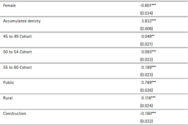
The explanatory variables of the model are: female, the individual’s cumulative average contribution density, generation cohort dummies, main contribution sector dummies, age, age squared; and the following are the macroeconomic variables: evolution of GDP, informality rate, female participation rate, and the interaction between female and female participation rate.
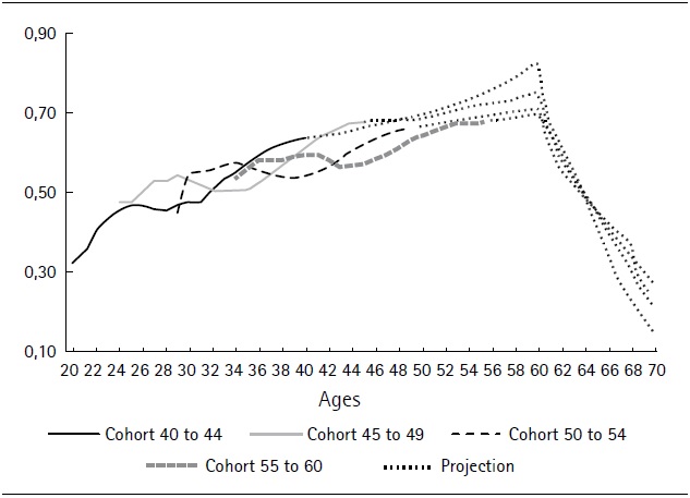
The cumulative average contribution density, for each period t and for each individual i is the ratio between the number of months that the person actually contributed to social security as a dependent worker in the period from April 1996 to t-1, over the total number of months in the same period. We define the binary cohort variables by age groups as of January 2017 from 40 to 44 years old (omitted category), 45 to 49 years old, 50 to 54 years old, and 55 to 60 years old. The contribution sector dummy variables follow the social security agency´s categories: Industry and Commerce (omitted category), Public, Construction, Rural, and Housekeeping Services.
Various specifications of the model were estimated. The final specification was the one that best predicted the evolution observed in the 2011 - 2015 period and yielded a reasonable evolution from 2016 onwards.7 Under our preferred specification of a variable that reflects past contributions, that is, including the individual’s cumulative average contribution density, the model correctly predicts 77% of the observations in the 2011 – 2015 period.
We should mention that not including a variable that has past information on the individual’s contributive behavior only predicts 51% of observations correctly, which reinforces the idea that past contribution is a key regressor to accurately forecast future. We subsequently applied a threshold to translate the predicted probabilities. We selected a threshold of 0.6 by also testing which was the best predictor in the sample period (2011 - 2015). The projection of the density of contributions results from multiplying the explanatory variables by the coefficients estimated in the probit model in table A.1 in the Appendix. It is worth noting that given that the modelling objective is to achieve the best possible projection and not to explain the role of a certain variable of interest on the probability of contributing to social security, the endogeneity considerations of the explanatory variables are irrelevant. Besides, given that several explanatory variables are included, it is possible that the sign of some of these variables may seem counter-intuitive, but it should be taken into consideration that we are comparing them with respect to very particular cases. That is to say, the group that meets all the omitted characteristics: men under 45 whose main contribution sector is Industry and Commerce as well as other aspects.
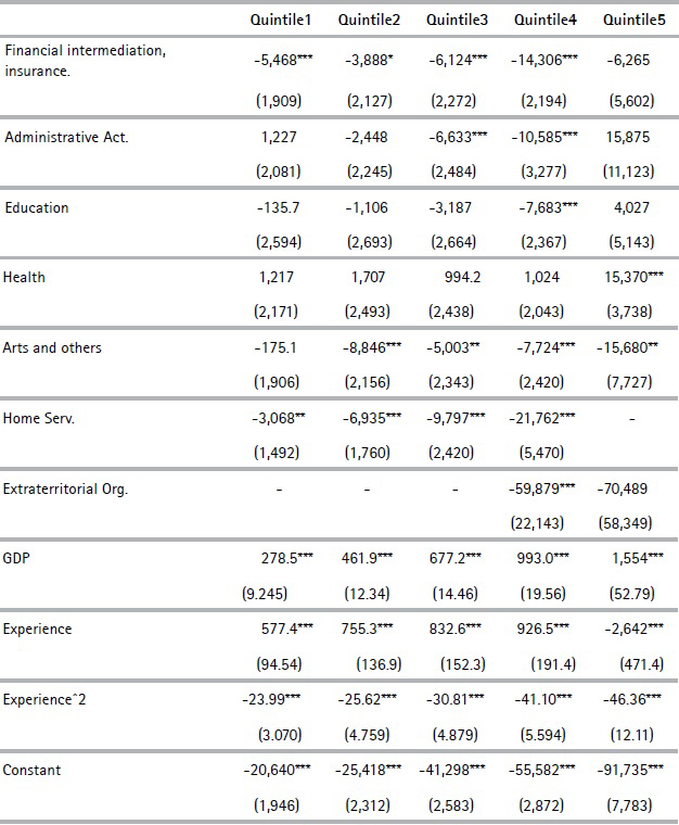
From 2016 onwards, we project GDP growth, female activity, and informality rates for 2046 for three macroeconomic scenarios (Table A.3 in the Appendix). We construct the base scenario under the assumption of a 3% GDP growth [in line with Güenaga, Mourelle and Vicente (2013) and Dassatti and Mariño (2014)]: a 2% increase in wages and a 3.5% return rate on constant prices of the individual savings fund (FAP). Likewise, we assume a gradual reduction in the labor supply gap between men and women of approximately 20% by the end of the period with a corresponding informality rate of 21%. The random effect is incorporated to the projections by adding a term  to the projection equation that generates a standard random variable with a 0 mean, and
  is the panel level standard deviation of the regression.8
Individuals’ behavior in the labor market significantly changes by the age of sixty when retirement becomes an option (at least for those who have met the contributions requirements). Therefore, it is not sensible to use the projection model described in the previous section for ages over 60. For these ages, we chose to replicate the evolution of the contribution density observed by gender and contribution sector for a random sample of 40,000 individuals who were between 60 and 70 years old in 2016 and apply this evolution to the projected trajectory for the sample of individuals currently aged 40 to 60 in our sample. Even if the behavior of individuals from our cohort of interest might change relative to what has been the behavior of older cohorts from age sixty onwards, we believe this approach yields a more reasonable evolution than the results from extending the probit model to older ages.
Administrative records are only available from April 1996 onwards. In order to compute monthly contributions prior to this date, the social security agency requires witnesses who can testify that the individual actually worked in a certain firm in a given time period. To determine the years of contributions prior to April 1996, we envisage two options: First, we use the information from the administrative records regarding the start date of the job the individual had by April 1996. We assume that since that date the person contributed without any interruption, and that s/he did not have another formal job prior to that date. This may underestimate the years of contributions the social agency will recognize especially for those who were close to forty in 1996 and can provide witnesses. For this reason, we also consider another option and choose the maximum years of contributions yielded by the two. The second option consists of considering the observed contribution density during the 1996-2002 period for each individual and applying that value since the person was 21 years old (age at which the majority of the population entered the labor market in the nineties according to Household Surveys) until April 1996.
Below we present the contribution projection for the different cohorts (spotted line) up to 70 years old for the base macroeconomic scenario.
B. Income model
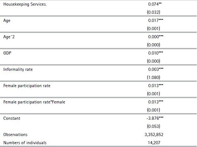
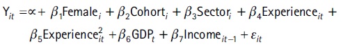
In order to estimate individual’s i annual income at time t, we propose a linear regression model with random effects that includes the following explanatory variables: female dummy, five-year age cohorts’ dummies, economic sector dummies according to ISIC classification, experience, experience squared, annual income in t -1, and GDP. The estimated income equation is as follows:
 (2)
(2)
Where  and vi is an individual random effect which is constant through time.
Following Berstein et al. (2006), we define the variable experience as the number of years contributed at time t. We estimate five separate models, one for each income quintile.9 Quintiles are calculated considering income between 2013 and 2015 at constant prices. Income is projected solely for those periods in which it is projected that workers will contribute to the social security system. Similarly to the contribution projections, for 2016 onwards, the random effect is incorporated by adding a term  to the projection equation that generates a standard random variable with a 0 mean and when
  is the panel level standard deviation of the regression.
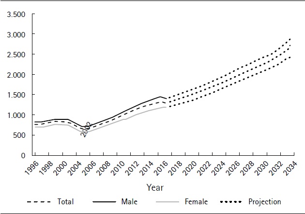
The figure below shows the evolution (and projection in dotted lines) of income by gender. It should be noted that the graph considers the evolution of income only for individuals who continue to contribute to the social security system. In this sense, the further ahead in time, the fewer individuals continue contributing, and those who do so belong to the younger cohorts and have the best contribution and income profiles. We present the coefficients of the estimated model for each income quintile in Table A.2 in the Appendix.
Source: Authors´ own computations derived from social security data.
Figure 3 Monthly wage projections in the base scenario (2017 average in US dollars)Note: the graph considers the evolution of income only for individuals who continue to contribute to Social Security. The further ahead in time, the fewer individuals continue to contribute and the better their income profile.
C. Reconstruction and projection of funds in the individual savings accounts and annuities
Firstly, for each individual in the sample we reconstruct the history of the contributions made to the individual account, which depends on the personal contributions earmarked for this pillar. They are related to each person’s income level and the choice of voluntary affiliation to the AFAP provided by Article 8 of Law 16,713. As we mentioned before, there is an administration fee charged by the AFAP, and a collective disability and death insurance premium.
The sample contains information about the date of affiliation with the AFAP for each individual and whether they chose to affiliate under the option provided by Article 8 of Law 16,713 but does not inform about the administrator chosen or assigned to them. Using information published by the Central Bank, we construct an average AFAP of the system (AFAP-System), calculated from the relative monthly participation of each administrator in the FAP. In this way, we calculated the average monthly quota of the AFAP-System between 1996- 2005, which reflects the historic average rate of return of the system as well as the administrative fees paid and disability and death insurance premium.
Based on the information from the BPS administrative records, we compute the individual’s average gross contribution to the savings pillar and subtract commissions paid, thus obtaining the net contribution to the FAP. From the quotient between the net monthly contributions and the average quota value of the AFAP System, the number of FAP shares (“cuotas”) that are acquired monthly by each worker are estimated. Thus, when valuing the number of shares acquired by the worker, at any given time, we obtain the total amount of savings in the individual account. For the projection, we assume an average yield of 3.5% measured in indexed price units (UI), which are equivalent to 1.5% over the evolution of the average wage. We assume that the expected performance of the accumulation sub-fund is identical to that of the retirement sub-fund.
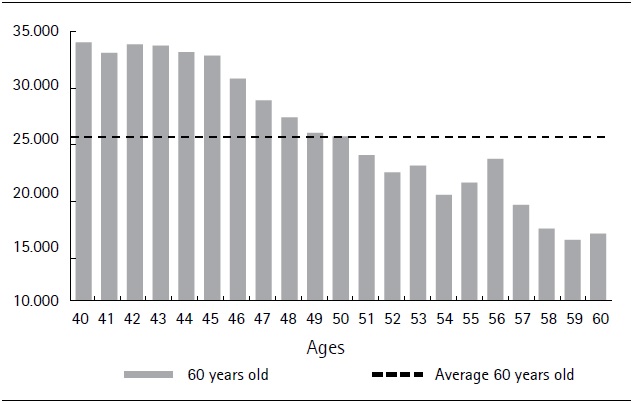
Figure 4 shows the projected FAP at age 60 for ages in January 2017 (horizontal axis). We can observe the “cohort effect” in relation to the specific situation within each age subgroup in the sample.
Source: Authors´ own computations derived from social security data.
Figure 4. Projected FAP at age 60 (2017 average in US dollars)
The age bracket in our sample contains individuals who were of different ages at the time when the multi-pillar system was introduced. This results in them having a different total number of years’ contribution to their individual savings accounts. Those close to 60 by January 2017 will have contributed a maximum of 21 years to their individual savings accounts: on average 80% less than those in their forties.
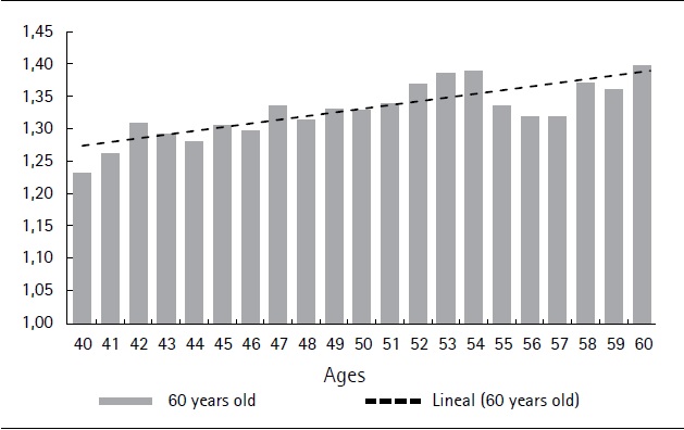
Based on the ratio between the FAP estimated at 60 years old and the sum of gross contributions to the individual, savings accounts at constant values (updated by the Consumer Price Index), we obtain a measure of the return of the contributions to this pillar (before paying for administration fees). According to our estimates, the average ratio at 60 years old for the entire sample is 1.33, which implies that, on average at this age, the FAP is 33% higher than the sum of gross contributions to this pillar.
Figure 5 shows that this ratio is increasing with the person’s age. This evolution indicates that older cohorts benefited to a larger extent from the high rates of return on Unidades Reajustables (unit value that is periodically adjusted according to the evolution of wages) registered until 2004, which we do not expect to recur in the future. This partly compensates for the shorter contribution of older individuals and thereby helps explain the low variation in replacement rates among cohorts.
Source: Authors´ own computations derived from social security data.
Figure 5. Ratio between FAP at age 60 and gross contributions to individual savings accounts by age (%)
According to our estimates, 29% of the cohort under study will never contribute to the individual savings pillar (AFAP). In turn, those that are expected to contribute for more than 30 years represent only 13%.
Regarding the calculation of life annuities (RVP for its Spanish acronym), we use the mortality tables published by the Superintendence of Financial Services, part of the Central Bank of Uruguay (SSF-BCU), at the beginning of 2017. This happened at a time during the public consultation on modifications to the individual savings scheme promoted by this institution.10 The tables published by the BCU include the update and dynamization of mortality tables, an increase in the reference population, and a better adjustment of the surcharge for the risk of survival. The update and correction of the probability of generating a pension for a family member in the event of the death of the RVP holder also represents an improvement relative to the previous tables. Likewise, for the calculation of the RVPs, we decided to use the current technical interest rate, which was set at 1.5% in UR by the SSF-BCU.11
V. Results
A. Years of contributions in the baseline scenario
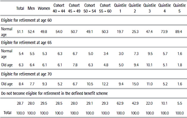
Table 2 presents the distribution of retirement ages when individuals retire as soon as they become eligible (immediate retirement), which is our baseline scenario. To present the results in a clearer way, we choose to analyze the situation of each individual in the sample with respect to their possibilities of becoming eligible for retirement at three different ages: 60, 65, and 70. An individual can retire at age 60 (“the normal age”) provided s/he has contributed for thirty years. If s/he has not done so at 60 years old, but does before the age of 65, for simplicity we assume s/he will retire at 65. In addition, if the person has accumulated between 25 and 29 years of contributions at age 65, we assume they retire as part of the old age regime. Furthermore, under this regime, a person can retire at age 70 if s/he has contributed for between 15 and 24 years. Estimates for years of contributions take into account special computations and the bonus contribution years per child for women.
Table 2. Distribution of retirement ages in the baseline scenario (%)Note: Calculations in Table 2 refer to our base macroeconomic scenario. Both the optimistic and moderate macroeconomic scenarios also project that, on average, 51% of the sample will become eligible for retirement at sixty. The main difference by scenario is observed for those who become eligible at 65 years old: 7.2% in the optimistic and 3.9% in the moderate. This is because the projected macroeconomic growth for 2017 onwards would have a greater impact on contribution densities projected at ages above 60 given the age structure of the sample. Therefore, the percentage of individuals who are not likely to retire from the PAYG scheme varies from 24.6% in the optimistic scenario to 30.5% in the moderate.
Source: Authors’ own computations based on social security records
We estimate that 51% of the workers would be able to retire at age 60. This estimation is higher than that projected by Bucheli et al. (2006, 2010) using administrative records for the period 1996 – 2004: 38 and 41.3%, respectively.
This could be explained by the sustained economic growth, lower unemployment rate, and decreasing informality rates observed during more recent years, as well as the bonus for the contribution per child introduced by Law 18,395 in 2008. Indeed, the percentage of workers not contributing to social security decreased significantly from 40.7% in 2004 to 24.7% in 2017 (the average informality rate in the 1996-2004 period considered by previous studies was 41.1%).
Men exhibit a slightly more favorable prospect in terms of their retirement although the gender gap seems to have significantly reduced in the last decade due to both bigger increases in the percentage of women contributing to social security as well as the 2008 reform that granted women an additional year of contributions per child (up to five). Also, there is a slightly better situation for the youngest cohort. On the other hand, we also observe that 28.7% of our sample would not be eligible for retirement in the PAYG scheme even at age seventy. About 60% of individuals who are not expected to retire by the pay-as-you-go scheme will accumulate five years’ contributions or less. These individuals are likely to be covered by the non-contributory pension although it currently targets individuals living in households with extremely low income.
B. Replacement rates in the baseline scenario
A pension replacement rate is the defined as the pension entitlement divided by labor income . It can be defined in several ways, especially depending on the labor income considered. The most popular measure uses the wage earnings of the year prior to retirement. In this paper, we analyze the ratio considering two earning periods: average earnings from the last year the individual worked and their average working life earnings.
Using earnings from the last year worked is more suitable to assess the pension system’s ability to smooth consumption between working and retirement periods, which is what a worker would evaluate when deciding whether to retire. Moreover, this approach enables us to make international comparisons as it is the most widely used ratio in the literature. In turn, the analysis of replacement rates expressed relative to average earnings throughout the emplo-yment history provides a better picture of the value of the pension in terms of the contributions the worker made during his active stage. It should be noted that this average only comprises periods with positive earnings.
We define the joint replacement rate as the ratio of the sum of the pension of the PAYG scheme and the annuity received from the individual savings scheme relative to total labor income for which the worker contributed. The PAYG rate considers the pension in that pillar in terms of the wage it covers, and the individual savings’ replacement rate is defined accordingly (annuities in relation to income devoted to individual saving).
In this section, we show our results in terms of replacement rates in the immediate retirement scenario discussed in Table 2, section 5.1. In addition to showing average replacement rates, in Table 3 we include median estimates to show to what extent average rates are sensitive to extreme values.12 We include the average contribution density and most frequent earnings quintile to emphasize that replacement rates at different ages are not comparable as they involve individuals with very different contribution and income profiles.
Table 3. Replacement rates in the baseline scenario (%)
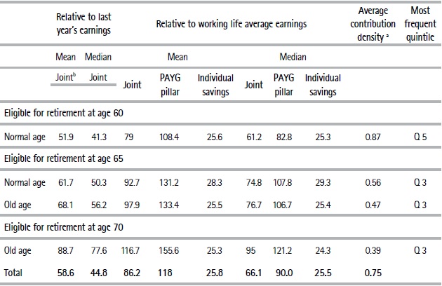
a Refers to the observed period in the sample: 1996-2015b Comprises both the pay-as-you-go and the individual savings schemes
Source: Authors’ own computations based on social security records.
Furthermore, it is worth mentioning that the effective replacement rates shown in this study should not be compared to technical rates used for the calculation of pensions. This is, firstly, because our replacement rate estimates consider the existence of minimum and maximum pension amounts. Secondly, it is because when the pension is calculated by the BPS, technical rates are applied to the average wage earned in the last 10 years, and the maximum of the average wage earned in the best twenty years is increased by five percent. Instead, as we already mentioned, to compute effective replacement rates we consider the ratio between the estimated pension to average earnings from the last year worked in one case and average working life earnings in the other.
Average replacement rates are significantly affected by extreme values due to the high incidence of minimum pensions that we estimate 45% of the sample will receive. At the same time, 23% of those who will receive minimum pension declare particularly low wages (below the national minimum wage for 44 hours per week). It should be noted that we could not obtain good quality information on hours worked by the individuals in the sample. The low levels of declared income have a substantial impact on the averages calculated for the sample as a whole, which can be seen by comparing the means and medians of individuals who become eligible at different ages.
On average, those eligible for retirement at age 60 are expected to obtain a replacement rate of approximately 52% with respect to the average earning of their last year’s contribution. On the other hand, the replacement rate in relation to the average salary of the individual’s employment history is 79%. This is consistent with the fact that wages generally increase throughout working life, therefore pensions expressed as a ratio of the last year’s earnings are lower than when expressed as a ratio of working life earnings. Individuals eligible for retirement at age 60 on average present a high contribution density (87%) and mainly belong to the fifth income quintile.
The remainder groups that would be eligible for retirement at age 65 and 70 (with lower contribution density and income than those eligible at age sixty) have higher replacement rates due to both the higher incidence of minimum pension recipients and the higher technical rates that are applied when individuals are older at the moment of retirement.
Considering all those individuals who will at some stage be eligible for retirement, and relative to their last year of earnings, average replacement is estimated at 58.6%, and the median is approximately 45%. Likewise, replacement rates calculated using the average income of working life have an average of 86% and a median of 66%.
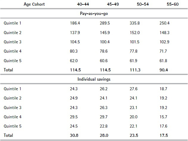
Focusing on the relationship between pensions and average working life earnings, we observe that the replacement rates of the PAYG scheme are on average above 100% for different ages and regimes (normal age and old age). This result is strongly influenced by the presence of the minimum pension beneficiaries, which we analyze in a following section. Therefore, those who manage to accumulate at least 15 years’ contributions would receive, on average, a pension above their working life earnings. This may suggest sustainability challenges that should be analyzed in future research.
Individual savings’ replacement rate estimates are on average 25%. They are expressed with respect to the wage covered by that pillar over the course of working life. We do not calculate the replacement rate relative to the last year of earnings for the individual savings pillar because it may be the case that workers do not contribute to their individual account during the year prior to their retirement. When comparing replacement rates for the two pillars, it is important to bear in mind that while the PAYG pillar also receives contributions from employers, the funds for individual savings only come from workers. Furthermore, the BPS provides other coverage, such as unemployment insurance, which does not have a specific financing. Finally, the replacement rates for the PAYG pillar do not consider the administration costs of the pension system, which are covered by the fee that AFAPs charge workers in the case of the individual savings scheme.
Figure 6 is a histogram showing the joint replacement rate (comprises both PAYG and individuals’ savings pillars) computed in terms of the last year’s earnings.
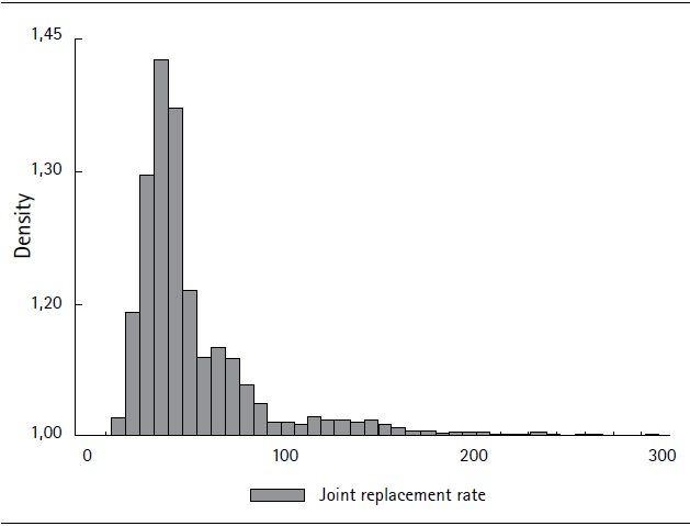
Source: Authors´ own computations based on social security records.
Figure 6. Histogram showing joint replacement rates calculated relative to the average wage in the last twelve months of contributions
Although it is difficult to compare studies across and within countries due to the different assumptions involved in each exercise, we conclude that Uruguayan replacement rates do not seem to differ much from those estimated for the average of OECD countries and other specific studies available for Chile.
OECD (2013) estimates a replacement rate of approximately 54% for middle-income workers of 34 member countries, which to some extent is comparable to our replacement rate of 51.9% estimated for those eligible for retirement at age 60 and relative to the last year’s earnings. However, it should be taken into account that OECD (2013) assumes individuals exhibit continuous contributions for forty years (i.e. no informality or unemployment spans).
According to our estimates, Uruguayan replacement rates that calculated the last year’s earnings seem to be slightly higher than those computed by Bernstein et al. (2006) for the average of Chile’s affiliates (44% in relation to last month’s and the last three years’ wages). As for replacement rates computed using the average working life earnings, according to Berstein et al. (2006), Chilean replacement rates are estimated at 121%. Chile requires men to retire at age 65, and the study also considers zero income during periods without contributions when computing average income. Our estimated replacement rate of 79% at age 60 did not include zero income periods when computing average working life earnings, but if we did the same, this estimate would rise to 131%. It should also be taken into account that we only have information on wages from 1996 onwards, that is, we lack information on the older cohorts’ first years of work, and this can result in overestimating average working life earnings.
Another study on Chile carried out by Paredes and Díaz Fuchs (2013), estimates replacement rates based on average income and pensions rather than on individual results. In this case, the results for retirement at the legal age result in an average gross replacement rate of 81%, with respect to working life earnings for both men and women. This is in line with our estimates for Uruguay (79% at age 60).
C. Impact of the minimum pensions benefit
According to the social security agency, 28% of the individuals who retired in 2015 received the minimum pension. It is reasonable to expect this figure to increase from 2016 onwards as those who contribute to the multi-pillar system begin to retire. This is due to the high percentage of workers with income lower than $48.953 (pesos as of January 2017) that voluntarily chose to assign 50% of their contributions to the individual savings account (Article 8, Law 16,713). As such, the amount of contributions to the PAYG pillar significantly decreased and that makes it more likely for workers to receive a minimum pension.
By 2017, the minimum contributive pension was $9,930 (approx. US 350 dollars).13 We assume this minimum evolves in line with the variation in real wages: an increase of 2% per year. According to our projections, minimum pension recipients would reach 45% of those eligible for retirement (70% of those expected to receive a minimum pension chose to assign half of their contributions to the individual savings pillar (Article 8, Law 16713). As mentioned before, this has a significant impact on average replacement rates.
Our findings suggest that there is a significant percentage of individuals who have high contribution densities and a particularly low monthly income (possibly explained by declaring only a few working days per month), and who would therefore qualify for a minimum pension. We estimate that 34% of those who would become eligible for retirement at age 60 would obtain the minimum amount: this percentage is higher for women (39.7%) than it is for men (29.3%). This proportion is even higher for those who become eligible for retirement at 65 years old and reaches 84% for those who would only be able to retire at 70.
According to our estimates, beneficiaries of the minimum pension on average duplicate the pension they would have received if no minimum existed. Nonetheless, the current system of access to minimum pension does not provide sufficient information to evaluate whether this benefit is targeting the poorest.
Table 4. Minimum pension recipients (%)
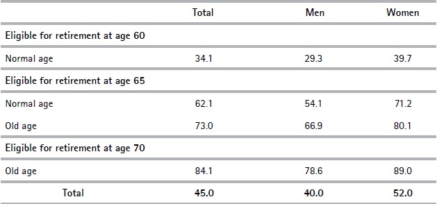
Source: Authors’ own computations based on social security records.
Following Decree 233/017, if we add the annuity derived from the individual saving accounts to the resulting pension from the PAYG to determine whether the individual would qualify for a minimum pension, the percentage of individuals who would receive a minimum pension would drop from 45% to 38%. However, the average replacement rate remains barely unchanged (58.4% relative to last year’s earnings and 85.6% relative to average lifetime earnings: compared to 58.6 and 86.2 reported in Table 3). This corresponds to the fact that the projected amount of annuities for the individuals who would no longer receive a minimum pension are expected to be very low.
D. Analysis based on socioeconomic characteristics
Table 5 shows the average replacement rates by gender, income quintile, and contribution sector for individuals who are expected to be eligible for retirement at age 60. Women exhibit lower participation rates and lower wages than men. These factors have a negative influence on eligibility for retirement and the expected pension amounts. However, because of the introduction of the one-year contribution per child scheme and the existence of minimum pensions, the projected replacement rates suggest that women will on average achieve higher replacement rates than men at the PAYG pillar and, therefore, also higher joint replacement rates. The computation of pensions in the individual savings scheme considers different mortality tables by gender, which reflects women’s higher life expectancy. This means that, for the same total savings, women have to finance a longer period of pensions than men, which results in lower amounts.14
Table 5.Replacement rates for those eligible for retirement at age 60 by characteristic
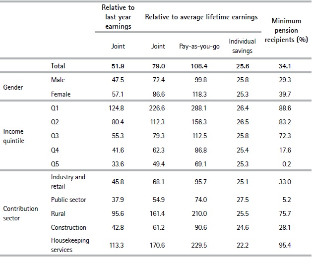
Source: Authors’ own computations based on social security records.
Pensions play a significant redistributive role; with substantially higher replacement rates at lower wage levels. Average rates among quintiles range from 124.8% in Q1 to 33.6% in Q5 relative to the last year’s earnings. These patterns correspond with the significant incidence of minimum pensions in Q1, Q2, and to a lesser extent Q3. Overall these results show that the PAYG pillar plays an important redistributive role for those who become eligible for retirement.
According to our estimates, workers in rural and housekeeping sectors have the highest replacement rates: around 100% relative to the last year’s earnings. Again, this fits with the large percentage of workers from those sectors that will receive a minimum pension when they retire (95% and 76%, in housekeeping and the rural sector, respectively). We argue that this is both due to low wages in these sectors and a high percentage of undeclared income (note that only individuals expected to be eligible for retirement at age 60 are considered in Table 5). Indeed, the Household Survey provides information on the percentage of undeclared income: the primary sector and housekeeping services in 2017 were the sectors that had the highest percentage of workers who stated that they did not declare social security for a percentage of their income.
Overall, replacement rates in the individual savings scheme do not show substantial differences. Most variation in joint replacement rates for gender, quintiles, or sectors is explained by differences in the percentage of minimum pension recipients.
Comparing replacement rates by age cohorts is particularly relevant given that in 2016 the first workers covered by the 1996 reform began to retire. A group of these workers, who called themselves the “cincuentones” (those in their fifties), argued that they would receive lower pensions compared to slightly older workers (not covered by this regime) and to those younger than them and under the same social security system. This triggered a partial reform in 2017 that allowed the cincuentones to abandon the multi pillar system and have their pension calculated as 90% of the pension they would have obtained under the PAYG system, which was in place prior to 1996.
In order to compare replacement rates between different age cohorts, we believe it is not desirable to express them relative to the average lifetime working life income because administrative data including income is only available from 1996 onwards. Therefore, for the older cohorts (ie. those aged 55 – 60 in 2017), we do not consider the income they earned during earlier stages of their careers. In turn, for those aged between 40 and 44 in 2017 we are likely to have data that covers almost their whole work history. For this reason, we consider that the relevant replacement rates that should be compared between different age groups (given the information available) are those expressed relative to the last year and relative to the average of the wages earned between age 40 and 60.
Table 6 breaks down average replacement rates by cohorts and quintiles using the two types of replacement rates. The results show that prospects for those in their fifties in terms of replacement rates are not that different to those of younger cohorts with similar income levels (joint replacement rates for those in Q5 are similar among age cohorts). The reason why we do not find significant differences is because even if individual savings replacement rates are lower for those in their fifties (this cohort had less time to grow their funds in the individual savings scheme), the PAYG pillar weighs significantly more in the joint replacement rate and there is no clear pattern between cohorts in this pillar. Indeed, when comparing replacement rates relative to the last year’s earnings, older cohorts in Q5 exhibit slightly higher joint replacement rates due to the PAYG pillar while when replacement rates are computed relative to wages earned between age 40 and 60, these are slightly lower. Overall, we conclude that the individual savings pillar plays a minor role in terms of its contribution to the joint replacement rates for all the age cohorts that were analyzed.
Table 6 Replacement rates at age 60 by cohort and quintile (%)
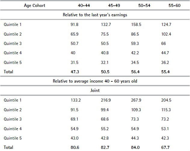
Source: Authors’ own computations based on social security records.
E. Sensitivity analysis
Replacement rates under different macroeconomic scenarios show two types of behavior. On the one hand, when considering the last year’s earnings, replacement rates decrease as macroeconomic conditions improve. This is explained by the fact that wage growth projected towards the end of individuals’ working lives is higher in the most favourable scenarios. Average rates decline by about eight percentage points, from an average of 64% in the moderate scenario to 58.6% and 56.6% in the base and optimistic scenarios, respectively. In terms of replacement rates in relation to average working life earnings, we observe the opposite behaviour. That is, they grow under the most favourable scenarios, implying a greater correlation between contributions over the entire working life and the resulting retirement. Average rates in the extreme scenarios increase 10 percentage points from 82.9% to 92.2% and from 64.6% to 69.5%. In these scenarios, we also estimated the number of people receiving minimum retirement benefits, assuming a minimum retirement growth of 3% and 1%, respectively for the optimistic scenario and moderate scenarios. In the moderate scenario, we estimated that 41% of the individuals eligible for retirement would receive the minimum pension, while 49% would do so in the optimistic scenario. Overall the main conclusions remain unchanged.
As a robustness check, we calculate replacement rates under the assumption that individuals’ income from 2016 onwards grows at an annual rate of 2% in real terms (provided they continue contributing to the social security system); thus, we ignore the income model described in Section 4.2. Replacement rates do not differ significantly from those reported in Table 3 (they are slightly higher relative to the last year’s earnings but slightly lower relative to working life earnings). Under this scenario, 47% of those eligible for retirement would receive a minimum pension.
We calculated the effect of a one percentage point decrease in the variable administrative fee charged by the AFAPs on the individual saving accounts replacement rate and an increase of one percentage point in the rate of return of the Fondo de Ahorro Previsional (FAP). The base macroeconomic scenario was applied in both cases.
We estimate that a reduction of one percentage point in the administration fee charged by the AFAPs will have a positive effect of 0.9 percentage points on the rate obtained by this pillar, while an increase in the rate of return of the same magnitude will increase the replacement rate by 2.4 percentage points. The limited effects estimated can be explained by the age profile of the cohort analyzed, for whom the potential effects of these parametric changes have a short-term impact: i.e. the last years of their work history. As expected, when analyzing the results after splitting them by smaller cohorts, we can see that the younger workers have been impacted the most by these exercises. A decrease in one percentage point in the administration fee the younger members of the sample were charged would imply an average increase in the replacement rate of 1.5 percentage points at age 60. Furthermore, an increase of equal magnitude in the projected rate of return would result in an increase in the replacement rate of 4 percentage points.
F. Replacement rates in the deferral scenario
In this section we estimate the effect the replacement rates have on deciding to postpone retirement for five years under the baseline macroeconomic scenario. We did this for a subgroup (43.6% of the sample) that is expected to have accumulated at least 30 years’ contributions at age 60 and for whom the contribution model projected they would continue to contribute at least until age 65. The results are presented in the table below.
Table 7. Comparison of replacement rates between immediate retirement at age sixty and deferred retirement until age 65
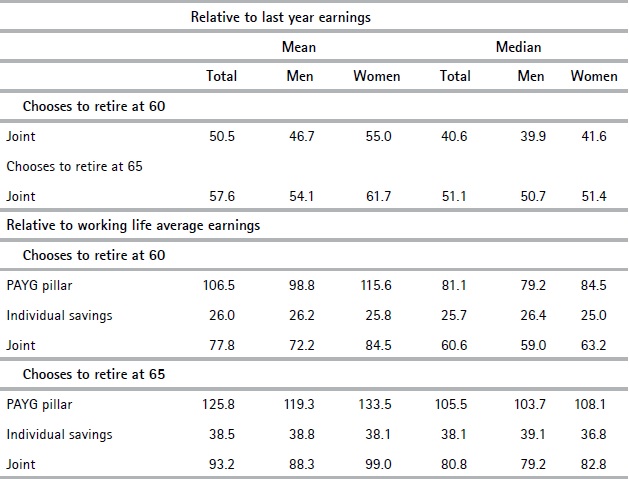
Source: Authors’ own computations based in social security records.
We estimate that the joint replacement rate measured with respect to the income of the last 12 months would increase on average by approximately 7 percentage points if retirement was postponed for five years (increasing from 50.5% to 57.6%).
The decision to continue working results in an average increase in pensions of 41% in real terms. However, the subgroups’ labor income is also projected to increase in real terms during those years (18% in real terms). This attenuates the increase of the replacement rate calculated using the last year’s earnings. Within this subgroup of individuals with a high contribution density, it is expected that 29.8% would receive the minimum pension if they retired at age 60, whereas if they postponed their retirement until age 65, this percentage would be reduced to 18%.
With regard to the replacement rate measured in terms of the average income of the individuals’ employment history, the joint rate would increase by 15 percentage points from 77.8% to 93.2%. That is, if individuals who accumulate at least 30 years’ contributions at age 60 continued to work until age 65, they would have a replacement rate of almost the average income earned during their working life.
Individual savings´ replacement rates under a scenario where individuals postpone their retirement until age 65 are estimated at 38.5%. This is in line with rates computed by Durán and Pena (2011) for Uruguay using household surveys.
Overall, our results suggest that the PAYG pillar has only mild incentives to defer retirement. This is not only related to technical rates but also to the incidence of minimum pensions. Alvarez et al. (2010) suggest incentives for postponing retirement are low compared to advanced economies. Also, Camacho (2016) argues that the premia added to technical replacement rates for each additional year of service relative to the minimum required for a given age (0.5%) is insufficient from a financial-actuarial perspective. It should be mentioned that while in Uruguay technical replacement rates increase by 3 percentage points for every additional year of deferred retirement (and additional year of contribution) in the PAYG pillar, pensions increase by 10.4 percentage points in the United Kingdom, 8.4 percentage points in Japan, and 8 percentage points in the United States (OECD, 2013).
VI. Conclusions
In this paper, we estimate eligibility for retirement and replacement rates of the Multi-Pillar security system in Uruguay for a cohort of salaried workers using a random sample of individual social security records.
The main results in terms of access to the contributive system show that there is a significant degree of polarization: while approximately half of the cohort would become eligible for retirement in the PAYG pillar at 60 years old, almost 30% would not be able to retire even at age 70. Most of the latter are expected to accumulate less than five years’ contributions in their working life.
With regard to the adequacy of benefits, although we acknowledge the difficulty of making international comparisons, we believe that our estimated joint replacement rate for the multi-pillar system at age 60 with respect to last year’s earnings (52%) is comparable to the OECD’s average (54%), according to OECD (2013), and higher than the minimum suggested by ILO (40%). It is important to consider that pensions in Uruguay are indexed exclusively to wage inflation, while according to OECD (2013) most countries do so relatively to consumer price inflation. Thereby, two countries with similar replacement rates at the moment of retirement may exhibit divergent trajectories if compared years after retirement.
Although our results indicate significant differences by income quintiles in terms of access to the contributive system, once individuals are eligible for retirement the system has a marked distributive profile. The existence of a minimum pension and the very recognition of years of contributions per child generate an important redistributive effect on the transition from active to passive life, which is shown by high replacement rates in the PAYG pillar for the lower quintiles. In future research, it would be interesting to assess the overall impact of the pensions system on inequality.
Our finding that 45% of those eligible for retirement would receive a minimum pension also points to the relevance of addressing challenges regarding informality both in terms of the percentage of workers who contribute to social security and the amounts they declare. It should be highlighted that this finding could only be obtained thanks to the use of individual administrative records. The fact that for a relatively important part of workers the declared income is smaller than the minimum wage suggests the need to revisit the contribution incentives according to actual labor income. Also, minimum pensions imply implicit subsidies to the PAYG pillar that should be quantified and their ability to target poverty assessed. Eventually, the role of the contributive and non-contributive pillars should be revised.
Overall, our results suggest that the PAYG pillar’s incentives to defer retirement are mild. In the same vein, Alvarez et al. (2010) and Camacho (2016) have pointed out challenges regarding incentives to postpone retirement because of the current technical replacement rates. As for the individual savings pillar, we conclude that this pillar plays a minor role in terms of its contribution to the joint replacement rates. This is not only the case for older workers who contributed to the multi-pillar system for a few years but also for younger workers whose entire work history is covered by it.
When comparing results by age cohorts, we conclude that there are no significant differences between the average joint replacement rates estimated for individuals currently aged 49 and those aged 50-60, even when we break down the results by income quintiles. This discussion is particularly relevant for policy issues since, in 2017, a law was passed to allow the “cincuentones” to be subject to conditions similar to those prevailing prior to the 1996 reform. In practice, the implemented changes delay the maturation of the multi-pillar system and just perpetuate the previous regime the solvency of which was questioned; thus, higher financial pressure was imposed on the system.
This study analyzes coverage and retirement-income adequacy of the Uruguayan social security system. Some of the estimations in this paper reinforce the ever-present need to assess the sustainability of the PAYG pillar in the medium term. In this sense, our finding that average replacement rates in this pillar relative to average working life earnings exceed 100% is a matter of concern. Analyzing the sustainability of the pension system should be addressed in future work as Uruguay has reached almost full coverage if both contributory and non-contributory schemes are considered and demographic tensions are expected to become even more challenging in the future. Indeed, the analysis of the sustainability of pension systems is likely to become part of a global research agenda as many countries are beginning to face similar demographic challenges.