


 English (pdf)
 Article in xml format
 Article references
 Send this article by e-mail
 Cited by SciELO
  Cited by Google
  Similars in
SciELO
Similars in
SciELO  Similars in Google
 Permalink
1.Introduction
The existence of socioeconomic differences between the members of a society are inherent to all modern societies in fields such as education, occupation, income, and prestige, among others (Rodríguez et al. 2020; Leo et al. 2016). Socio-economic stratification plays a fundamental role in public policy for the planning, design and implementation of specific programs to reduce social and economic inequality (Zhou and Wodtke, 2019).
Socio-economic stratification is not without controversy and disagreements (Fujihara, 2020; Tang, 2017; Haer, 1957), since proposing valid indicators implies connecting theories and quantitative or qualitative methods, which allow theories to be operationalized. According to Haug (1977, p. 51), clear theoretical proposals are the main “obstacle” in the measurement of social stratification, since these are “complex, contradictory, diverse”. Thus, the criterion considered to classify individuals is not unique and some methodological approaches are distinguished. In general, three approaches are prominent: quantitative, qualitative and mixed approach (Silva, 1981). In the first approach, which is also used in this article, indicators or classifiers are built using statistical methods in order to classify individuals, households or housing based on variables that collect individual, household or housing characteristics. For example, these variables are considered to be related to the education and occupation of the head of household, housing characteristics, income level and purchasing power.
The Principal Components Analysis (PCA) is commonly considered a suitable method for the construction of indicators as it reduces a large number of variables to a smaller number of uncorrelated linear combinations of these variables. These are called principal components and they represent the data as closely as possible (Mori et al., 2016). However, despite the benefits of the PCA and its broad-ranging use, this methodology presents a limitation when it comes to building indicators as the variables must be linearly related and numerical (Linting et al., 2007).
Given the qualitative and quantitative nature of the variables normally used for social stratification, the PCA assumptions are not met. Linting et al. (2007) propose an alternative named Nonlinear Principal Components Analysis (nonlinear PCA) which allows the incorporation of numerical and categorical variables and nonlinear relationships. Variables are quantified by the optimal scaling process, so that variance is optimized. Optimal scaling is based on the alternating least squares procedure, an iterative process that uses the previous quantifications to estimate the following quantifications, until converging to the solution (Krijnen, 2006; Kuroda et al., 2013).
In non-linear PCA, it is important to evaluate the stability of the results obtained. However, defining stability is a controversial issue already under discussion. Ferrari and Manzi (2010) argue that stability is an unfinished issue and that until now no conclusive and definitive results have been presented. For example in Gi (1990), the stability of an analysis method is defined as the analysis’ degree of sensitivity to variations in the data or parameters of the model. According to the same author, a solution is stable if a small change that is unimportant in the data, the model or technique leads to a small and unimportant change in the results. In this article, stability is the degree of sensitivity of the results against changes in the data. Small changes in the data should lead to changes in the level of the results of the analysis. Efron and Tibshirani (1993); Linting and Van der Kooij (2007) present an option for the verification of solution stability by means of non-parametric bootstrap.
In this context, this article builds an indicator for socio-economic stratification for Ecuador at provincial level7. In this country, socioeconomic stratification plays a fundamental role in public policy, for the planning, design and implementation of specific programs, to exemplify, the identification of the beneficiaries of conditional income transfer programs. It is also a tool used in demography, sociology, political science and marketing, among other areas of knowledge.
The contribution of this article, alongside the socio-economic stratification indicator, is that it is obtained through the non-linear PCA method. To the best of our knowledge, there are no studies using this methodology and our aim is mainly empirical.
The data used correspond to the Population and Housing Census (2010). The selected variables are related to characteristics of the head of household, the possession of household goods and the characteristics of the housing. For the stability analysis of the results obtained from the non-linear PCA, the bootstrap method mentioned in the previous paragraph is applied.
The article is organized as follows. After this introductory part, Section 2 contains a brief literature review. Section 3 describes the database and methodology used. In Section 4 the results are presented and discussed. Finally, Section 5 shows the conclusions of the work.
2. Brief Literature Review
Social stratification consists in classifying people or groups of people in a society (Kerbo, 2017). Although, academically, European social scientists such as Max Weber, Karl Marx, Wilhelm Dilthey, Émile Durkheim are recognized as the pioneers in the study of stratification and social class (Lemos, 2012), the idea of classifying individuals dates back to advanced ancient societies. For example, Kamakura and Mazzon (2013) mention the social classes of Athens (citizens, and slaves), Sparta (spartiates, perioecis and helots) and Ancient Rome (patricians, noble plebeians and plebeian gentes) to argue that the existence of well-established social classes with clearly defined characteristics to differentiate them extends to antiquity. The same authors state that this classificatory notion is still used today but with different terminology.
Although the construction of groups implicitly implies the legitimacy of the differences in the distribution —of wealth, goods or income—, ignoring individual heterogeneity would create a false illusion of equality and temporal stability of socio-economic conditions (Kerbo, 2017). It is an undeniable fact that the unequal distribution of goods favors a group that concentrates not only on wealth, but also on power, and leaves those who are not as important a part in this division at a disadvantage.
Even though from a normative point of view the acceptable level of inequality, as well as the deliberate delimitation of social and economic groups, are debatable, these facts are usually associated with social and political conflicts, which can even put democratic systems at risk (Acemoglu et al., 2015). In some way, the study of socio-economic stratification ratifies the existence of these differences (see Fujihara, 2020; Wu, 2019; Wright, 2005; Featherman and Hauser, 1976), however, the transparency of the imbalances in the distribution of goods and wealth provides information that allows reflection on the desirable structure of a society in terms of social and economic inequality. It also, depending on its members’ level of aversion to inequity, offers instruments to reduce inequality, to a greater or lesser extent.
3.Data and Methodology
3.1 Data
3.1.1.Description of the database
The data used in this article correspond to the Population and Housing Census (2010) conducted by the INEC, which provides the following general information: Ecuador, at the census date, had 14,483,499 inhabitants. At household level there were 3,815,527 households and 3,810,548 heads of household. The difference between household and house is that the word household is used to designate a person or a group of people who live under the same roof and share the food expenses, while the house is the space where people live, which is separated by walls or other elements covered by a roof (INEC, 2012).
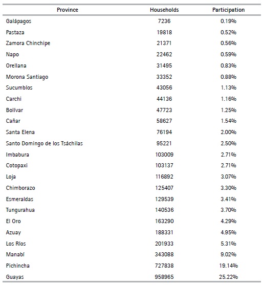
The information used in this paper relates to 3,802,566 households, in conjunction with information on housing and the heads of households. Variables at individual, household and housing level had to be used to make sure that the segmentation conducted collects as much information about Ecuadorian households as possible. In terms of provinces, Table 1 shows that the province with the most households in Ecuador is Guayas, with 958,965 households (25.22%), followed by Pichincha with 727,838 households (19.14%).
For the selection of variables, the initial criterion consisted of considering those variables8 that present the least amount of missing data, between 0% and 10%. However, in these cases, a simple imputation process was carried out; that is, the missing values of a variable were replaced by the average value of the units observed in the variable.
3.1.2.Categorization of variables
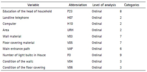
The nonlinear PCA method makes it possible to analyze a set of data with qualitative and quantitative variables; however, as the objective of this article is to obtain an indicator of households’ social stratification in the provinces, the variables are categorized in an ordinal way, which refers to changing the original scale of the variables in the Table 2, by turning them into ordinal variables. The categories are classified under the criteria of possession of goods and access to services that each category represents; i.e., the first category “1” is assigned to the lowest value categories under the criteria mentioned above, while the last category is assigned to the ones that present the best characteristics.
Table 2 Selected preliminary variables
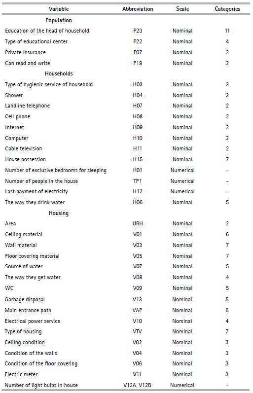
Source: Authors based on Data from the Population and Housing Census (2010)
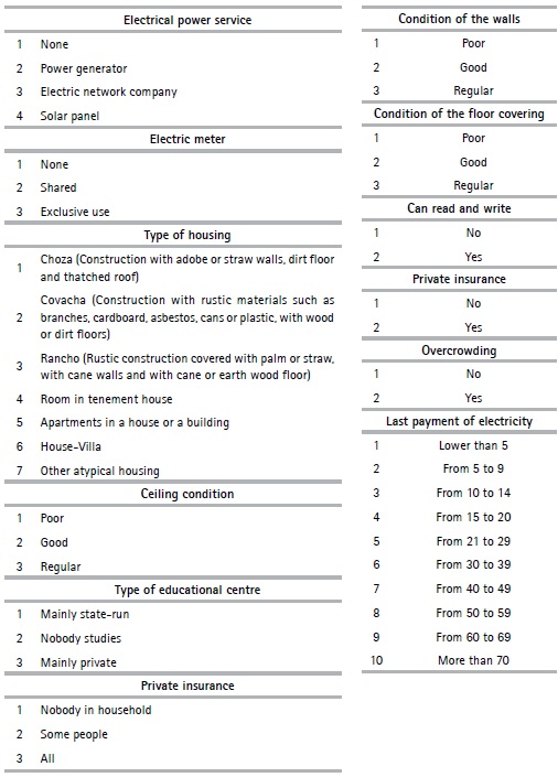
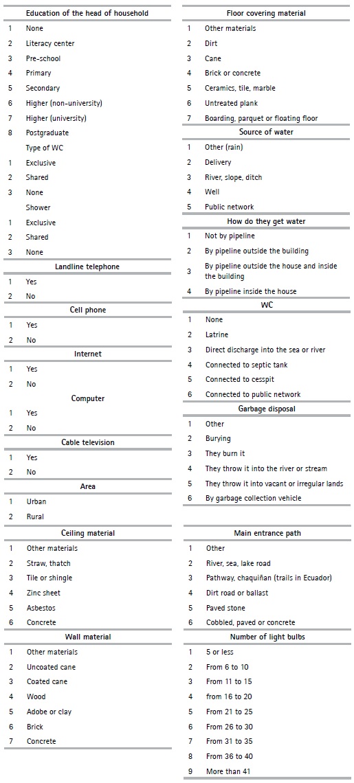
For example, if we take the variable area of Table 2, we assign “1” to rural area and “2” to urban area, since the rural area generally has less access to services than the urban area. In tables 3 and 4, the preliminary variables are presented with their respective categories.
Furthermore, in some cases, it was necessary to create the variables based on the census information; for example, the case of variable overcrowding, which was constructed from the general information of the household and the head of the household. Overcrowding refers to the relationship between the number of people in a house (TP1) and the space or number of available rooms (H01) (See Table 2). Since poor people’s access to resources is limited, the housing facilities they occupy tend to be less appropriate than those available for non-poor people, “1” is assigned to yes and “2” to no.
3.2. Methodology
The first version of the Nonlinear Principal Components Analysis (nonlinear PCA) method was described by Guttman (1941). Other contributions to this methodology were made in later years by Kruskal (1964), Shepard (1966) and Kruskal and Shepard (1974).
The nonlinear PCA is presented as a generalization of the PCA, since it makes it possible to incorporate qualitative variables, with ordered and unordered categories (ordinal, nominal), and to discover and treat nonlinear relationships between variables. Mori et al. (2016) present nonlinear PCA as the result of minimizing two loss functions, rank and homogeneity analysis, both of which are the subject to restrictions, in conjunction with the optimal scaling. In order to find the solution, one has to minimize several parameters of the loss function simultaneously using the alternating least squares technique (Mori et al., 2016).
Young (1981) expresses that optimal scaling is a quantification technique that assigns numerical values to the categories of the variables, under the restrictions of the analysis level of the variable (numerical, ordinal and nominal) and turns them into a vector of optimal scale. On the other hand, while minimizing the loss function, the solution must be found with several parameters simultaneously. The Alternating Least Squares (ALS) algorithm is used as a tool to solve this minimization problem. The ALS algorithm is an iterative process based on the alternation, where first the loss function for the first parameter is minimized while the remainder is kept fixed, and then the loss function for the second parameter is minimized, keeping the remainder fixed, etc. (Krijnen, 2006; Kuroda et al., 2013).
3.2.1. Bootstrap Method
In the context of the nonlinear PCA, the nonparametric bootstrap procedure is employed to evaluate the stability of the nonlinear PCA solution (Linting and Van der Kooij, 2007). This procedure incorporates the random bootstrap with replacement, which is based on the original sample called principal sample and consists of obtaining B bootstrap samples from the principal sample (Efron, 1997; Efron and Tibshirani, 1993). The bootstrap samples obtained are balanced; that is, it is guaranteed that the initial observations appear exactly B times in the B samples (Linting and Van der Kooij, 2007; Davison et al., 1986).
Subsequently, the analysis (CATPCA algorithm) is performed for each of the bootstrap samples, which results in B values for the quantifications of categories of the variables. B bootstrap values for each of the nonlinear PCA results are obtained, forming a bootstrap distribution, from which a confidence interval can be calculated. These same confidence intervals are used to analyze the stability of the results (Linting and Van der Kooij, 2007; Markus, 1994; Efron and Tibshirani, 1993). In this work, the confidence intervals will be obtained for the outputs of the algorithm, i.e. for the optimal quantifications for the categories of the variables.
The quantifications of the categories of selected variables and the bootstrap samples along with the quantifications of the principal sample are recorded in order to create the confidence intervals (a confidence interval is associated with a level of confidence at (1) 100%). Linting and Van der Kooij (2007) present the construction of the confidence intervals for the quantifications obtained through percentiles.
In the context of nonlinear PCA, the quantifications with small intervals, obtained from bootstrap samples indicate how stable the optimal quantifications are; in other words, if the quantifications of the bootstraps samples are not very different, the solution is considered stable (Linting and Van der Kooij, 2007).
This study employed the CATPCA algorithm, included in the SPSS statistical program, which was introduced in version 10 of SPSS in mid-1999 (Meulman et al., 1999). The patch used in this work is IBM-SPSS 23 and the complete algorithm is followed by Mori et al. (2016); Washed (2004); Fernando (2014).
4. Results and Discussion
4.1. Results
4.1.1. Selection of variables
The CATPCA algorithm is applied for each province with the preliminary variables defined in the previous section (See Table 3 and Table 4). This is done in order to maximize the variance explained by each principal component within each province. Using this criterion, several similarities are identified when analyzing the variables that contribute most to the variance of the first component, and a pattern is found within the 24 provinces. Table 5 presents some selected variables.
4.1.2. Result analysis
Based on the selection of variables described in the previous section and once the sample design was obtained for each of the analyzed provinces, the CATPCA algorithm was performed to acquire the optimal quantifications of the categories of variables and to analyze the variance explained by the components. At this point, the bootstrap procedure is applied with B=1000, followed by the presentation of a stability analysis of the results.
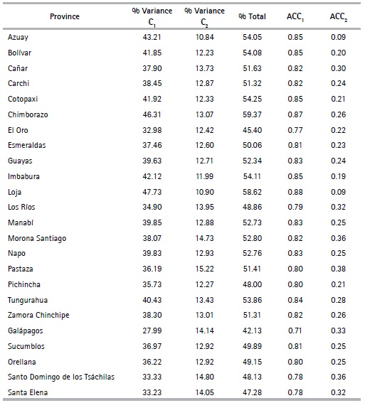
Variance analysis
The results obtained include the variance that is recorded for the first (% Variance C1) and second (% Variance C2) components, along with the total variance (% Total) (See Table 6). It was also concluded that the variance explained by the two principal components ranges between 45% and 59%. The province whose first component explains the highest percentage of the data is Loja, with 47.73%, and the province that has the lowest variance is Galápagos, with 27.99%. For Pichincha, the first component has a variance of 35.73% and for Guayas, a value of 39.63%. The variance calculated for the second component is observed to be greater than 10% in all provinces.
To determine the reliability in the internal consistency of components, the Cronbach alpha coefficient9 of the first (ACC1) and second component (ACC2) is used (See table 6).
The value of the Cronbach alpha coefficient in all provinces is greater than 0.7; thus, it can be concluded that the first component is reliable, depending on how well the information is represented. The Cronbach alpha coefficient of the eigenvalue associated with the total eigenvalue presents values greater than 0.8; that is, when the two components are used, the total reliability increases. It is also important to mention that the total variance explained in the first results of the execution of the CATPCA algorithm with the preliminary variables (See Tables 4 and 3), is lower in all provinces with respect to the results obtained in this section with the final variables. This is due to the selection of the final variables under the criterion of greatest contribution.
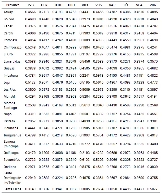
Table 7 presents the analysis of the explained variance for selected variables in the first component for each province. For example, the education variable for the head of the household (P23) in the province of Chimborazo shows greater variance, with a value of 52%, in Morona Santiago, this variable has a value of 25.09%. On the other hand, in Galápagos, the landline telephone variable (H07) has the lowest recorded variance with 12.09%, while in Bolívar, it represents 47.40%. In the province of Sucumbíos, the landline telephone variable (H10) presents the lowest value compared to the rest of the provinces which can be explained by the fact that access to a telephone network in the Eastern provinces is rather poor- with a value of 38.79%, and in Loja 46.75%. The area (URH) of house location in Santa Elena has a value of 8.3% and 59.88% in Chimborazo. The wall material (V03) in Sucumbíos has the highest value (61.03%), while Tungurahua has the lowest (10.92%). Santa Elena presents a variance of 26.63% and Chimborazo a 64.26%. In Galápagos, the main entrance path variable (VAP) presents a variance of 6.89%; owing to the fact that in this province, the main entrance road for over 65% of the dwellings is paved, cobbled or concrete. In the characteristics related to wall (V04) and floor (V06) conditions, Morona Santiago presents the lowest values at province level: 22.89% and 25.67% respectively. The highest values are in Guayas (48.74%) and Santa Elena (50.77%). A similar analysis can be performed of the results of the second component.
Table 6 Cronbach’s Alpha-Variance
Source: Authors based on Data from the Population and Housing Census (2010)
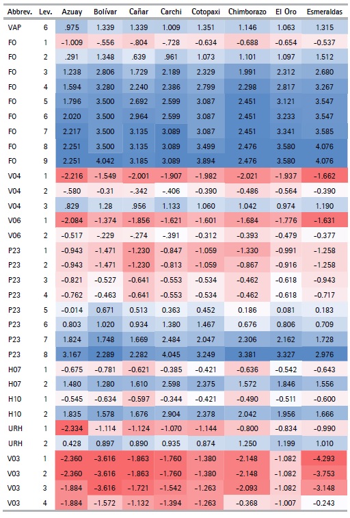
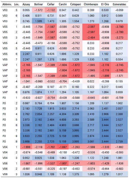
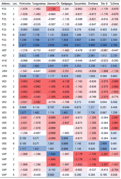
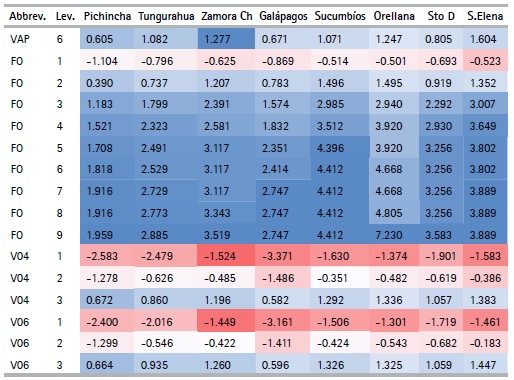
Quantification analysis
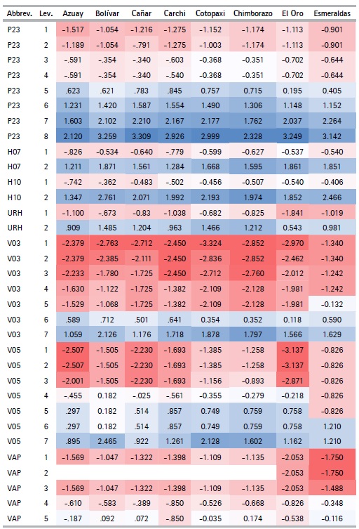
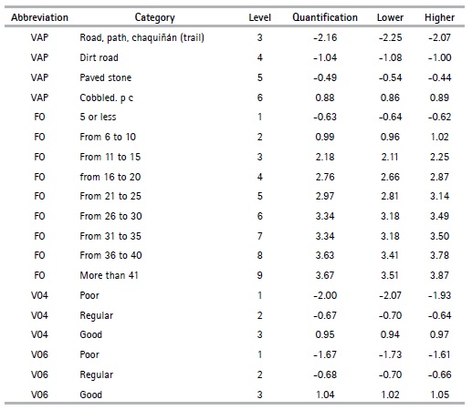
The CATPCA algorithm applied for each province with the selected variables (See Table 5) makes it possible to obtain the optimal quantifications of the categories of variables (See table 8). Using these results, the outcomes can be analyzed. The variables describing the materials of the walls (V03) and floor (V05) of the house, along with those that describe their condition (V04, V06 respectively) present the lowest value quantifications for the first categories when compared to the quantification of the first categories for the rest of the variables.
We can also see that the quantifications obtained are similar (not equal) for the different provinces, with the exception of the number of light bulbs variable (FO), which in each province takes values that are quite different from each other. For example, in Pichincha the category of the number of lightbulbs variable take values in the range of -1.104 to 1.959, while in Orellana it ranges between -0.501 to 7.230. This effect is due to the difference in frequency of the categories of this variable in each province.
Another exception is seen in the adobe or clay category in the wall material variable (V03), since in the provinces of Los Ríos, Manabí, Morona Santiago, Napo, Pastaza, Sucumbíos, Orellana, Santo Domingo de los Tsáchilas and Santa Elena the quantifications are positive, while in the rest of the provinces they are negative, thanks to the low frequencies these provinces present for this category. Finally, the categories with null frequency have a null quantization. This characteristic is presented in the second category of the variable, main entrance path to housing (VAP), with alternatives such as river, sea or lake, since some provinces might not display housing with this characteristic due to their geographical location. The variable appears mostly for households belonging to the provinces of the Coast or the Amazon Regions, such as: El Oro, Esmeraldas, Guayas, Los Ríos, Manabí, Morona Santiago, Napo, Pastaza, Zamora Chinchipe, Sucumbíos, and Orellana.
Table 8 Quantifications by province
Source: Authors based on Data from the Population and Housing Census (2010)
Table 8 Quantifications by province (Cont...)
Source: Authors based on Data from the Population and Housing Census (2010)
Table 8 Quantifications by province (Cont...)
Source: Authors based on Data from the Population and Housing Census (2010)
Table 8 Quantifications by province (Cont...)
Source: Authors based on Data from the Population and Housing Census (2010)
Stability analysis (Bootstrap)
A stability analysis is shown below to complement the results obtained in the previous sections and to identify whether the quantifications are stable. In other words, the analysis must be robust to changes in the selection of data and given that the quantification process is considered an integral part of the analysis, the algorithm is applied for each bootstrap sample. If the quantifications are substantially different from the quantifications of the principal sample in the analysis of the bootstrap samples, the quantifications will be unstable. If the quantifications have small confidence intervals, this means that they are stable. Table 9 presents the quantifications (Quantification) obtained from the CATPCA algorithm, along with the lower (Lower) and upper (Upper) limits of each category obtained using the bootstrap method. Specifically, the stability analysis of the results obtained for the province of Guayas is shown. The study considers a total number of bootstrap samples within each province, with a 95% confidence level and the solutions are obtained in two dimensions. Considering the aforementioned criteria, it can be concluded that the quantifications obtained in the province of Guayas are stable, since the confidence intervals are small.
Table 9 Guayas - Quantifications and confidence intervals
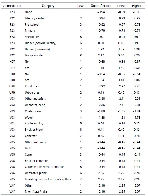
Source: Authors based on Data from the Population and Housing Census (2010)
4.2. Discussion
4.2.1 Analysis of national behavior
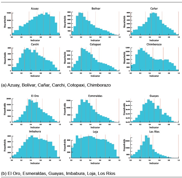
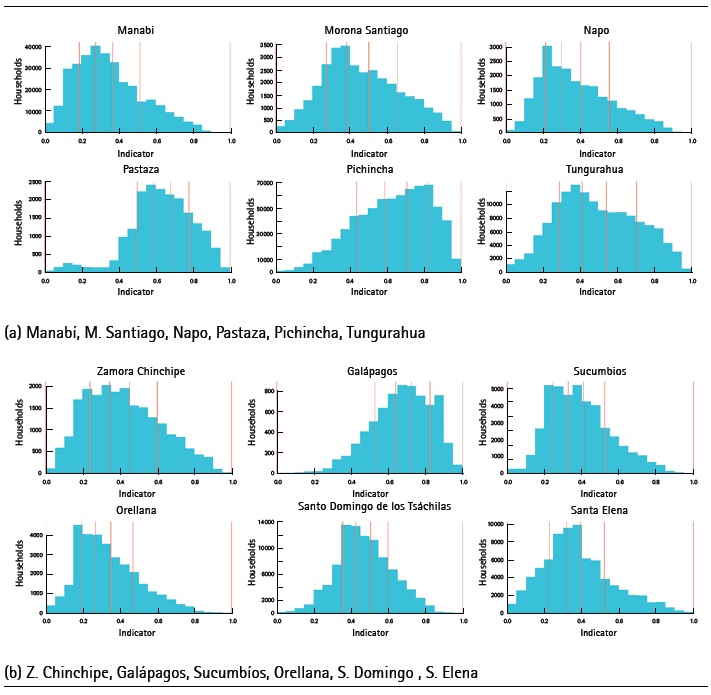
The indicators for each province are constructed based on the quantifications of the categories of variables in Table 5. Figure 2 displays the distributions of the indicators for Ecuador’s different provinces. The indicator values fall within the range of [0; 1] due to the rescaling performed; however, it is important to note that this does not mean that the indicators are comparable, as the quantifications of categories obtained for each province and with which the indicator is constructed with are different. To exemplify, for the variable head of the household’s education level (P23), the quantification of the first category —no education— in Pichincha is equal to -1.73, while in Sucumbíos it is equal to -0.96. The quantification of the last category, postgraduate, in Pichincha is equal to 1.88 and in Sucumbíos, it is equal to 3.63.
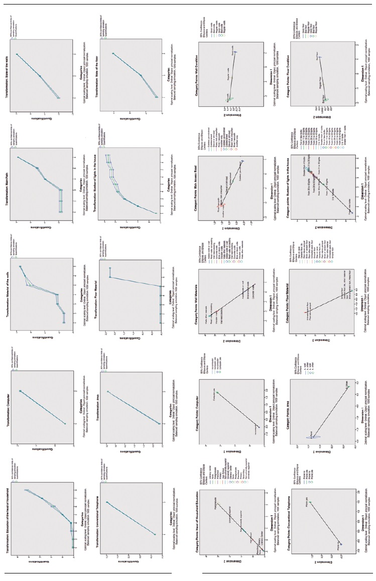
Figure 1 Guayas - Bootstrap(a) Initial Scale - Optimal Quantification (Quantifications, Upper and lower limits)(b) Component 1 - Component 2 (Quantification - Confidence Ellipse)
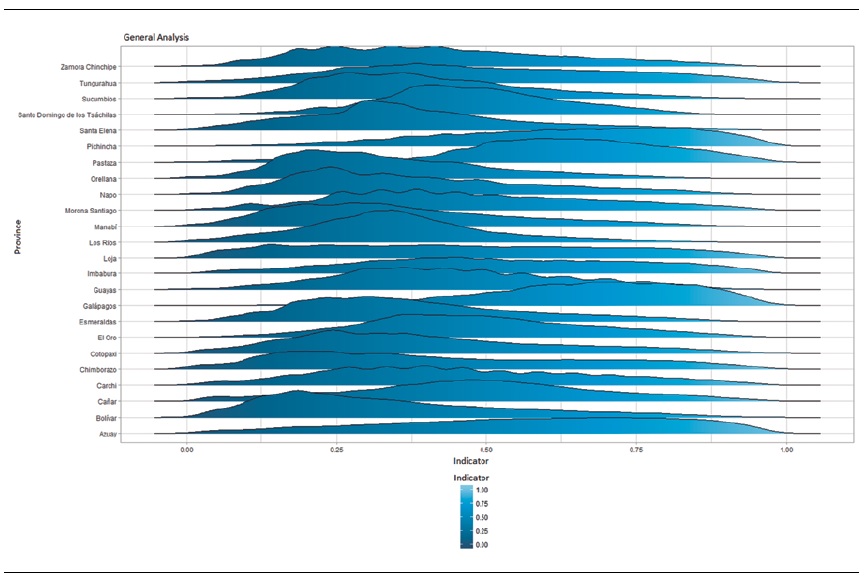
Once the socioeconomic indicators of each province have been constructed, a descriptive statistics analysis for each of these indicators is carried out. See Table 10. For the reasons stated above, the analysis to follow is not performed in a comparative context, but a descriptive context within each province. The average value for the socioeconomic indicator of households in the provinces of: Azuay, Pichincha, Pastaza and Galápagos shows high figures, whereas the lowest values appear for the provinces of: Orellana, Bolívar, Los Ríos and Manabí. At national level, the average values are in the range of 0.3350 to 0.673. On the other hand, the dispersion of the socioeconomic indicators of the provinces of Azuay, Chimborazo and Loja are high; while in Santo Domingo and Los Ríos the dispersion is low. The degree of dispersion for all provinces varies between 0.146 and 0.251 and, in general, it is high in all provinces. Moreover, Pastaza, Galápagos, Pichincha, Azuay and Imbabura have a negative asymmetry value; that is, the values of the household indicator tend to be located more on the right side of the average. In the rest of the provinces (See Figure 2), this coefficient is positive, so their distribution is concentrated on the left. This frame demonstrates that within each province a large percentage of households are below average. The result reflects the country’s unequal living conditions in the country and also suggests that there is a minority group of households with good socioeconomic conditions.
Table 10 Summary of indicators
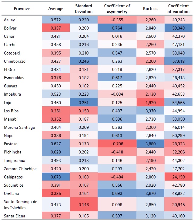
Source: Authors based on Data from the Population and Housing Census (2010)
The kurtosis coefficient for Los Ríos, Orellana and Pastaza is greater than 3, which implies that the distributions of the indicator are leptokurtic; that is, households are concentrated in the average. In the rest of the provinces this coefficient takes values of less than 3, indicating that there is a small concentration of households around the average. As the coefficient of variation makes it possible to compare the relative dispersion of the socioeconomic indicators of provinces, the greatest dispersion of the socioeconomic indicator is observed in the provinces of Bolívar, Chimborazo, Cotopaxi, Loja and Manabí. This reflects that households within these provinces present greater variability than in the rest of the provinces. Finally, in Pichincha, Pastaza, Galápagos and Santo Domingo de los Tsáchilas there is less variability among households.
Thus, the households within each province are grouped over quintiles, where the first quintile represents the households in worse conditions in terms of goods and services, while the fifth quintile represents the households in better conditions. In the Figure 3 and 4, the cut-off point of the quintiles is observed for each of the country’s provinces.
It is important to mention that the province of Galápagos is a nature reserve that is isolated to a certain extent thanks to its geographical position. Also, its main economic activity is tourism, which indirectly affects all sectors of the island’s local economy (Taylor et al., 2007). The above, together with the fact that it presents the lowest percentage of variance explained by the components (See Table 6), the general results for Galápagos are different from the rest of the country’s provinces.
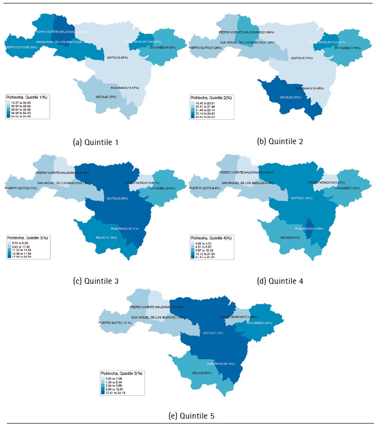
4.2.2 Distribution analysis of the indicator over quintiles
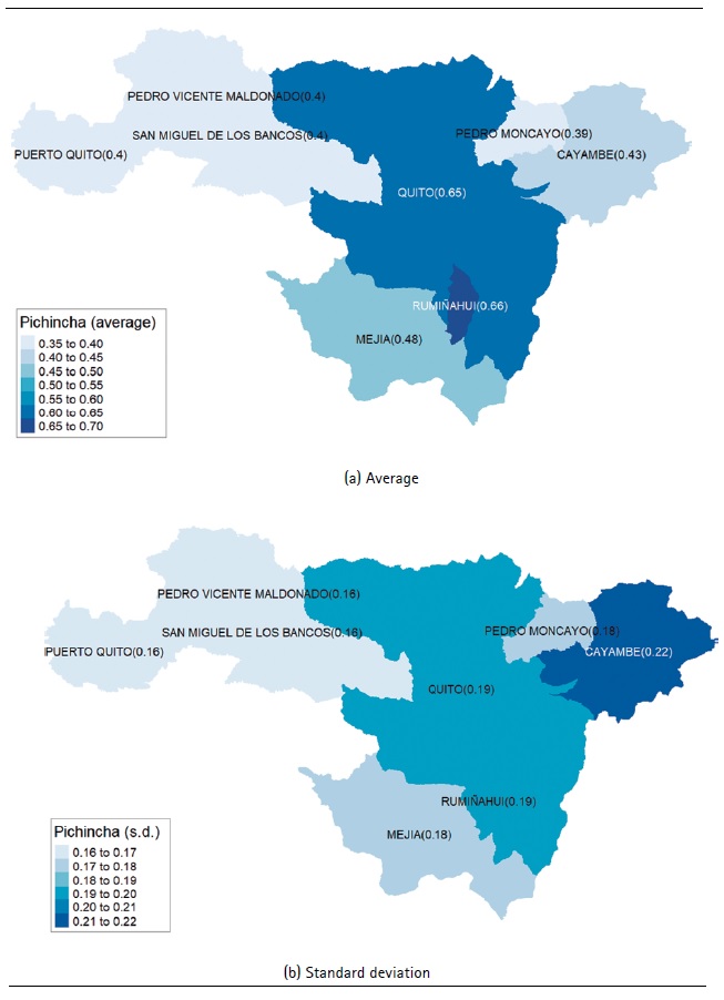
Given the importance of having a detailed description of the different quintiles within each province, their characteristics are presented for the particular case of the province of Pichincha.
Pichincha
The province of Pichincha contains about 19.14% of the country’s households distributed in 8 cantons. Figure 5(a) shows that the Rumiñahui canton has the highest average indicator value (0,66), followed by Quito (0,65). This implies that, in general, the households of these cantons have better living conditions. This could be explained by the fact that Quito, the capital of Ecuador, and Rumiñahui are strongly interconnected by geographical location, labor interests and economic activity between these two cities. On the other hand, Pedro Moncayo has the lowest average value (0.39). The households in this canton have the worst living conditions in the province of Pichincha. When analyzing Figure 5(b), the largest indicator dispersion is in the Cayambe canton (0.22), while the smallest dispersion occurs in Pedro Vicente Maldonado and San Miguel de los Bancos (0.16).
Figure 6 displays an analysis of the quintiles of the households belonging to Pichincha cantons. 64.66% of Pedro Vicente Maldonado’s households belong to the first quintile, which makes it the canton with the highest percentage of households belonging to this quintile, followed by San Miguel de los Bancos and Pedro Moncayo with 63.39% and 63.09% respectively. The main activities in these cantons are agriculture and tourism. At the other extreme, Quito and Rumiñahui have the lowest percentage of households within the quintile, with 16.65% and 15.57% respectively and the dispersion in each canton ranges between 0.08 and 0.12. Some 26.35% of Mejía households are in the second quintile, followed by Pedro Vicente Maldonado with 21.64%. The cantons with the lowest percentage of households in this quintile are Quito and Rumiñahui with 19.74% and 19,.5%, respectively. The analysis of the following quintiles is similar, since as of the third quintile, Quito and Rumiñahui have a higher percentage of households. Pedro Moncayo and Pedro Vicente Maldonado have the lowest percentage of households within these quintiles. The dispersion of Pichincha households within each quintile is low, except for the one belonging to the first quintile that has dispersions of up to 0.12. In the other quintiles, the dispersion fluctuates between 0.03 and 0.04.
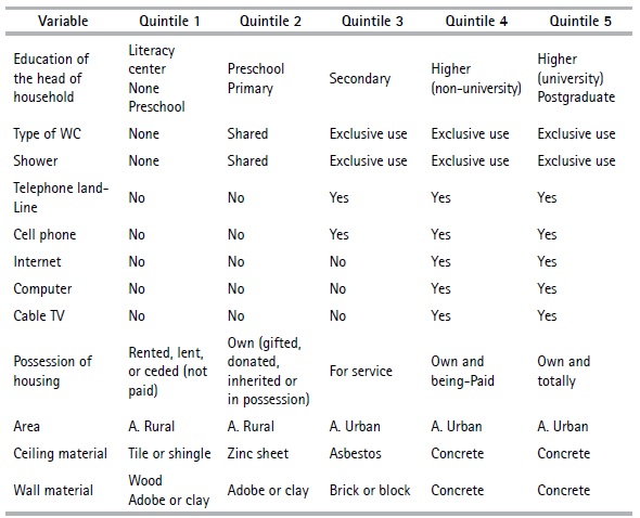
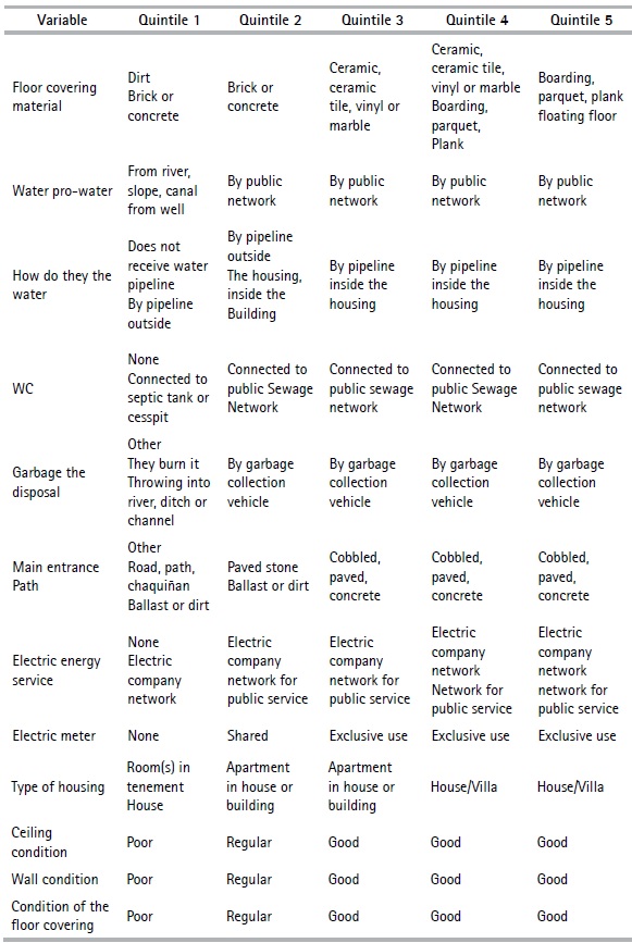
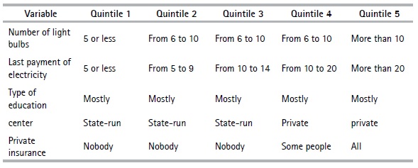
Table 11 presents the profile of the households belonging to each quintile. The characteristics of the first quintile consist of rented, lent or ceded housing or type of rooms in tenement house —which constitutes the majority— and those located in the rural area. The housing materials are tile, wood, adobe, and brick with poor conditions. They do not have basic services such as electric power, WC, garbage collection, landline telephone, internet, computer, cell phone and cable television. The head of household has a low level of schooling, none of the household members has private insurance, and they study in state-run educational centers. The households belonging to the second quintile are characterized by being in the rural area, with their own housing but inherited or ceded, the materials of the roof, walls and floor are zinc, adobe and brick or cement, respectively. These tend not to be in very good condition. They don’t have the basic services; the shower and WC is shared with other households and the level of education of the head of household is primary. The members of the households of this quintile conduct their studies in public educational centers and no one has private insurance. In the third, fourth and fifth quintiles, the households have a WC and shower for private use, as well as the basic services mentioned above. The housing of these households in these quintiles are their own, and tend to be apartments or houses that are in good condition, built with brick, block, concrete, ceramic tile or parquet materials. The main entrance road is paved or concrete. Household members of the third quintile study in public centers and do not have private insurance. Those in the fourth and fifth quintiles study in private centers and some or all members of the household have private insurance.
5.Conclusions
This article built socioeconomic stratification indicators for provinces in Ecuador. The results of this analysis constitute a tool for the fields of economics, political science, demography, sociology and marketing. In economics, for example, the information on social strata is essential for designing and implementing public policies. We constructed indicators of socio-economic stratification at the provincial level, which reduce the variability of the indicators obtained with respect to those obtained in similar studies, also conducted in Ecuador. Another contribution of this article is the application of the nonlinear PCA that allows the incorporation of quantitative and qualitative variables.
Our results were subjected to a sensitivity analysis using the bootstrap method and in general, showed that they are robust. However, some categories presented a low frequency which ultimately lead to large confidence intervals. This issue could be solved by appropriately clustering these low frequency categories. Another alternative is to modify the scaling of the abovementioned categories by using different scale levels, such as ordinal spline. On the other hand, the main advantage of using nonlinear PCA, compared to other similar techniques, is that the optimal quantifications obtained from ordinal variables retain their ordinal property, which allows for a socio-economic stratification interpretation of indicators.
Regarding the socio-economic conditions, it can be concluded that the households located in the urban area display better conditions and greater access to basic services. Likewise, the education level of the head of household is a key factor when characterizing household quintiles and the results suggest that, in general, education positively affects social and economic conditions of both individuals and the households. The results also suggest high inequality among the provinces. In Guayas, for example, there is huge inequality between Samborondón and Colimes. A similar situation is observed in Pichincha with cantons like Quito and Pedro Vicente Maldonado. In light of these results, public policy should be focused on the education, both in quantity and quality, of the school-age inhabitants of the cantons in worse social and economic conditions. Likewise, public investment in the provision of basic services such as drinking water, sewerage, electricity, access roads and garbage collection should focus on the cantons that, as explained by their conditions, have been the most neglected.

