


 English (pdf)
 Article in xml format
 Article references
 Send this article by e-mail
 Cited by SciELO
  Cited by Google
  Similars in
SciELO
Similars in
SciELO  Similars in Google
 Permalink
1. Introduction
This paper presents estimates of the economic value of increases in the length of life for a large set of countries using life-cycle data on consumption, leisure, earnings, and mortality. Calculations use a model of the value of statistical life (VSL). This is the first study that uses life tables for all countries and combines them with data on economic variables to obtain estimates for each country. Considering values from the bottom up makes it possible to calculate income elasticities of the VSL directly, unlike previous literature which assumes values of income elasticities to calculate VSL for less developed countries through extrapolation, based on measurements for wealthier countries. Estimated values of gains in longevity have large orders of magnitude, which highlights the value of investing in health. The main contribution is to estimate VSLs for all countries using a common database of mortality, to provide data which is as widely available as possible for consumption and work by age, and a coherent set of assumptions on preferences for intertemporal substitution. To obtain a consistent and comparable measurement of the gain in economic value from a longer life for all countries is key to advancing our understanding of the behavior of societies in relation to investments in prevention and expenditures in health care.
VSL calculations are more common for wealthier countries, whose governments employ estimates in regulatory proceedings. To obtain figures for other countries, the VSL for a wealthier country has been adjusted by national income and other variables (Jamison, et al., 2013); this approach is sometimes known as “benefit transfer” (Robinson, Hammitt and O’Keefe, 2019a). For example, Masterman and Viscusi (2017) use a VSL calculation of $9.6 million for the United States and estimates of income elasticities of VSL that are above 1 for other countries to conclude that values range from $107,000-$420,000 for low-income countries, $1.2 million for lower-middle income, and $6.4 million for upper-middle income countries.
Robinson et al. (2019a) searched the literature over a 20-year period and found studies for 15 countries, all of which are high- or middle-income. Using those results as data, they estimate a relation between income and VSL. They recommend the use of income elasticities between 1.0 and 1.4 to extrapolate existing results to countries with no studies and to use values of a life year that exceed monetary consumption to consider other life benefits. Both considerations are implicit in our calculations through the assumptions on parameters for elasticity of substitution and minimum consumption. In their calculations, an improvement of 1 in 10,000 in risk generates a willingness-to-pay (WTP) of $900 for the United States ($54,000 GNI per capita) and $300 for a country with a per capita GNI of $30,601.
However, a review by Hersch and Viscusi (2010) suggests an income elasticity of the VSL of approximately 0.5 to 0.6; that is, an increase in income is reflected in higher VSL less than proportionately. An overestimated income elasticity (for example, a value of 1 when the true value is 0.6) understates the VSL for lower-income countries. Estimates of VSL in segmented populations are affected by the wage offer faced by individuals (Viscusi, 2018). Even if preferences towards risk are identical for all, the WTP for increases in longevity is affected by the potential monetary gains. In international comparisons, societies with flatter risk-earnings tradeoffs have lower VSL.
The solution to the issue is not to improve the benefits transfer approach, but to estimate VSLs directly using risk and labor data that covers all countries. This is what this research does.
Estimates of VSL are usually classified as labor market, hedonic or revealed preference approaches, and stated preference studies. A typical application of the first approach uses data on wages and occupational risk, and characteristics of firms and workers, to identify the compensating differentials between jobs of different risk levels and thus calculate the VSL (Thaler and Rosen, 1976). A stated preference study obtains data through surveys; for example, a survey may inform the interviewees of the level of risk linked to an event and of a potential change, and ask for WTP (Knieser and Viscusi, 2019). Our approach falls into the hedonic class because it uses an observed relation between risk (survival probabilities at each age) and national income levels.
Murphy and Topel (2003) point out that much remains to be done to improve calculations of VSL and to link them with medical research and stress the need for data on lifecycle patterns of income and consumption, and on life expectancy. They also point out to the use of disease specific data; although this paper does not use the detailed information available in the Global Burden of Disease project (GBD; IHME, 2017), our approach can accommodate the analysis of specific illnesses. They also refer to data on health research (which we do not have), and on health and quality of life, on which we have partial information in the GBD database. Thus, while not all issues are treated, this research furthers the use of lifecycle data in economic and health variables.
Section 2 presents the methods used in the evaluation. Section 3 presents the arguments to select parameter values and the econometric estimations to calculate VLY and VSL, and Section 4 displays scenarios of improved longevity. Section 5 discusses potential improvements.
2. Material and methods
2.1 Model to evaluate gains in longevity
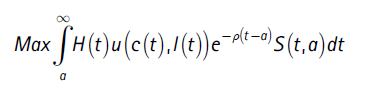
The economic model to assess longevity improvements is based on the hypothesis that people assign a high monetary value to a small increase in the probability of survival. As a result, they are willing to sacrifice some vital consumption in exchange for a longer lifetime. A formula to valuate health status was developed by Murphy and Topel (2006) and is the same formula applied to any asset in economic models.
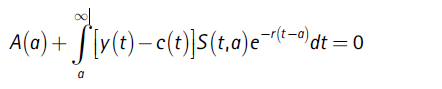
In equation (1), H(t) measures health status, c(t) is consumption of goods different from health services, .(t) is leisure, and S (t,a) is the probability that an individual in cohort . survives to date t. Parameter r reflects inter-temporal preferences and . is the interest rate at which the person can save or borrow. The time horizon is infinite, but the chances of survival are very low at ages just below 100. Income and expenditure must comply with a budget constraint, expressed in equation (2), in which variable . measures the value of assets.
 1
1
Subject to:
 2
2
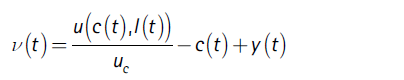
The solution to this problem produces the VLY, v(t), as the sum of the financial flow and the monetary valuation of utility in a period (equation 3). As an intuition on why the first term on the right side is interpreted as a monetary value, we can note that the numerator is an unobserved quantity, while the denominator is the reciprocal of the money required to buy additional utility; thus, the term is a price times a quantity.
 3
3
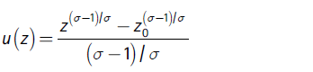
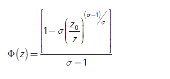
The model uses two assumptions concerning the period-specific utility function to facilitate the calculations. First, the relative demands for leisure and consumption are independent of a person’s level of wealth (zero income effects). Second, the utility function includes parameters relative to “survival consumption” (z0) and intertemporal substitution (σ). These assumptions are imbued in equation (4) and imply the surplus function Φ(z) in equation (5).
 4
4
 5
5
The variable Z is a composite commodity that adds consumption to leisure using prices as weights. This is possible because there are no income effects: Z = ZcC + ZII.The parameter σ of intertemporal elasticity of substitution plays a main role: if it has a value close to zero, lifetime consumption profiles do not change following alterations in the relative cost of consumption between periods; for example, unexpected, exogenous news of an increase in longevity does not alter planed consumption. An alternate way to express the implications of low σ is that consumption does not respond to the interest rate (the inter-temporal price of consumption). On the other hand, very large values of σ mean that consumers are not willing to sacrifice consumption to increase longevity.
The calculations of v(t) involve: (i) estimation of consumption, income, and leisure profiles using a cross-section econometric model; and (ii) selection of parameters of intertemporal substitution and minimum consumption through price theory and a review of the extant literature. The values of v(t), together with data on probabilities of survival (S) and disability (of which H is a function), and an assumption of the intertemporal discount parameter (ρ) are plugged into equation (1) to obtain the VSL.
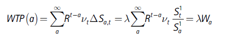
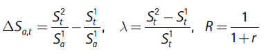
Willingness to pay (WTP) for an increase in longevity is defined as the difference in VSL under two different patterns of survival. The calculations are based on the discrete time version shown in equation (6). Superscripts 1 and 2 denote alternative survival scenarios. Timewise, the product of a change in survival probabilities at age α ( ΔSa t, ), the value of a life year and the discount factor Rt-a -generates changes in the WTP(α). This is the value of the increase in longevity ΔSa t, .
 6
6
A change in the lifetime distribution of survival probabilities can take an arbitrary form. Two scenarios are defined to measure reasonable levels of improvement. One is a homogenous improvement for all countries and age groups, the other assumes convergence towards the levels of the longest-lived countries. The first scenario is a shift proportional to all future ages, and can be described through a parameter λ.
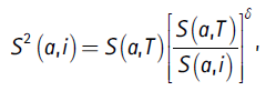
A second scenario follows a pattern of convergence in which all countries approach the longest-lived, in proportion to life expectancy; the country with lowest life expectancy improves proportionally more, the longest lived shows no improvement, and the rest show improvement that is somewhere in between. To construct this, counterfactual survival probabilities for each country and age, S2(a,i), are obtained by applying the following calculation, where T refers to the country with the highest life expectancy:
The VSL includes the variable H(t). H-health is approximated through data on Years lost to Disability (YLD), which is in turn based on disability weights obtained from the Global Burden of Disease database (Salomon, et al., 2015). This assumes that disability weights measure the loss in welfare due to a condition by decreasing the VLY.
A review of the causality framework exposes the potential bias of the results. As stated, it says that the survival patterns are independent of consumption-work decisions, rates of interest and discount, and disability patterns. If data were for individuals, these assumptions would be less acceptable because an individual who learns that she has an improved likelihood of survival or lower expected disability is likely to change her work-consumption decisions. The results below assume implicitly that, for populations, changes in survival probabilities arise in such a way that populations cannot respond quickly to them. Thus, estimates can be thought of as being short-term.
Aldy and Viscusi (2007) discuss the calculation of VLY and VSL by age. These studies usually define a hedonic wage equation and use a fatality risk variable determined by the remaining years of life. The VSL is also built as the discounted sum of VLY. However, a main difference with the calculation in this paper is that we do not estimate a wage equation. Instead, we assume a structure of preferences and impose parameter values that vary with per capita income. Thus, we have the equivalent of a hedonic wage equation in the relation between income and survival probabilities. It may be noted that we do not aim to estimate only one value of VSL, but rather a set of values, one for each country.
2.2 Data
This section explains the construction of variables used to calculate the VLY (equation 4): c, l and Y. The information comes from two classes of sources: labor, consumption, and health data are taken from international databases, while parameter values are obtained from extant literature and price theory criteria.
Health data come from IHME (2017), a rich database that contains information on mortality, illness, and disabilities for almost all countries. Consumption data are from the National Transfer Accounts Project; 23 countries are included in the analysis, using the most recent data (NTA, 2019; Lee and Mason, 2011). NTA data are mostly cross-sectional and not updated periodically for most countries. Labor data are from the ILO (2020), which has information on labor force participation for all countries in the NTA database.
The selection of countries is dictated mainly by data on individuals’ consumption by age. These are not produced directly in administrative or market process, and the way resources are distributed among household members is not homogeneous in relation to household size and structure. For example, increased longevity does not always imply longer working lives and the reasons are complex due to strong wealth effects on the demand for leisure and to the institutional environment for retirement (including social security and the internal arrangement of households in relation to multi-generational families). Improved data would provide consumption levels by individuals for several years.
For health, the GBD database (IHME, 2017) provides information on death rates and on years lost due to disability (YLD; WHO, 2018) by age.3The values of survival probabilities are obtained directly for 2017. The variable H is built as 1 minus the percentage rate of YLD by country and age.4
Leisure is measured using data on rates of participation in the labor market by age, which is available for most countries for several years. Data on hours of work by age is less common because it is produced from high-quality national labor surveys and relatively few have them; ILO data do not provide systematic information on hours by age. We calculate hours of work by age as the product of hours and labor force participation by age. To construct the variable on leisure hours we take the number of hours in a year minus the hours of work.
For earnings, NTA data includes variables by age group. Comprehensive global data sets to study earnings over the lifecycle are not available. To explore patterns across countries, researchers have selected countries with richer data. In a recent study, Lagakos, et al. (2018) focus on 18 countries with better data and, within that set, on 8 core countries with cross-sectional data over 15 years or more. However, even for that selected group, they focus on income from salaried work. The ILO and the World Bank data have information on earnings from different sources by sex, occupation, and sector, but have not produced harmonized data by age.
In sum, there are no systematic data on leisure, earnings, and consumption variables comparable in quality to the IHME health database. The NTA provides the larger sample of countries with harmonized data on earnings and consumption by age and determines the set of countries in the study. We use the more recent data from the NTA for each country; few countries have more than one year of data available, making it impossible to develop models with time effects.
2.3 Specification of consumption, earnings, and leisure profiles
A regression model is used to obtain values on expected consumption and income over the lifecycle and by age-group. Available data panels are unbalanced, less so for health data, but more so for labor data, and even more so for consumption data. This explains the strategy of calculating regression models to build life-cycle profiles of consumption, leisure, and labor earnings for each country.
The assumption is that consumption, income, and leisure profiles can be represented by a common model across countries and over time, and the regional parameters are useful to measure differences in behavior across countries. The heuristic is that the shapes of consumption, income and leisure profiles change slowly, and are stationary over time except for a shift in levels determined by national income levels and regional effects. The main argument against this assumption is that longevity increases productive age and time effects on the average consumption and income profiles. However, the lack of panel data for most countries and the long interval of time required to identify those effects precludes their identification.
The regression model relates consumption, earnings, and leisure (j=c,e,l), to powers of age (α) and regional dummies Index i refers to countries and
  refers to regions of the world. The error term uij is assumed to be independent of age and country
 , iid across countries). Time effects are not included, a decision dictated by data availability on consumption by age group.
The model provides consumption profiles over the life cycle in intervals of five years (α = 1,…,20) because that is the framework of NTA data. Thus, the profiles are assumed to have age coefficients common to all countries (βh), and regional effects (γhi). The choice of the order of the regression polynomial (h) is made on empirical considerations.
Equation (9) describes the models for per capita consumption, leisure, and earnings at each age α, and region i. The models include dummies for five regions, defined in part by the availability of consumption data: Latin America and Caribbean (Argentina, Colombia, Costa Rica, El Salvador, and Jamaica), Europe (Austria, Finland, France, Hungary, Moldova, Slovenia, Turkey, and United Kingdom), Asia (Cambodia, Singapore, South Korea, and Taiwan), North America (Canada and United States), and Africa (Ethiopia, Ghana, Nigeria, and Senegal). Estimates are weighted by population by age group for each country. For earnings, NTA data have variables for total labor income, and subcategories for employed and self-employment labor income. Here, we use the variable on total income. Calculations use values at ages 15 to 65 relative to the 30-49 age group.
 9
9
The estimated coefficients are used to obtain profiles of the variables for each region. For consumption and earnings these are multiplied by the per capita income of each country to obtain consumption and earnings profiles by country (equation 10):
 10
10
3. Parametrization and estimation
3.1 Parameter selection
In addition to the consumption, earnings and leisure profiles, the calculations involve six other parameters: the time discount rate (ρ), the interest rate (r), the elasticities of substitution between consumption and leisure, and between consumption at different points in time (σ), the parameter for minimum consumption (zo/z), and the number of hours over which the calculation is made.
Murphy and Topel (2006) use 1.1 for σ and 0.05 for zo/z. In a lower income country, a smaller gap between consumption and subsistence consumption is justified (i.e., a higher zo/z). This follows the meta-analysis of Havranek et al. (2013), which indicates that lower income populations are less likely to substitute consumption over time as they are closer to the minimum acceptable levels of consumption. It will be useful to investigate the role of the assumption on zo/z. On ., Havranek, et al. (2013) find average values of 0.5 in an evaluation of estimates for 104 countries. They find that richer households and households in countries with more developed financial markets show higher values of intertemporal elasticity. On the other hand, in a recent review of the literature, Low and Meghir (2017) refer to the “practice” of using σ at a slightly higher value than 1.
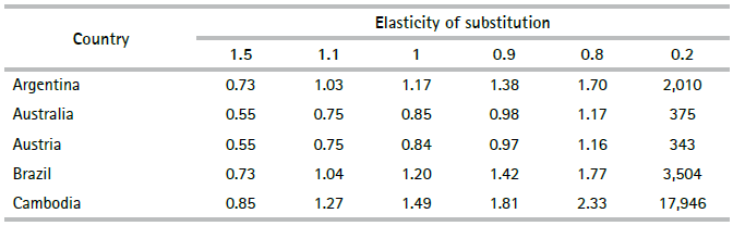
To support the selection of parameters, Table 1 shows estimated average values of one year of life relative to GDP per worker for a country for different combinations of σ and zo/z(this covariation has the same sign for all countries). When σ approaches zero, the value of one year of life reaches very high values; this is not meaningful because, if true, individuals place a lot of value on the possibility to live a little longer, the VSL is thousands of times higher than market income, but at the same time individuals are not willing to reduce consumption profiles by much. On the other hand, if the elasticity of substitution is large (say, 10), individuals’ may not care whether they consume in one period or another, the VLY approximately equals income, and individuals do not care about longevity. Note also that variations of the VLY near σ = 1.1 are not small because poverty (defined by high values of zo/z) reduces the value of longevity. Our analysis uses values of zo/z between 0.2 to 0.05; country-specific values are assigned linearly between those extremes according to GDP per worker. Thus, the wealthiest country has 0.05, and the poorest has 0.2; for example, the values for Mozambique, Chile, Spain, and United States are 0.20, 0.16, 0.11 and 0.05, respectively. For the elasticity of substitution, we use σ = 1.1 for consistency with other studies and because values far from unity lead to absurd counterfactuals (McCloskey, 1987). However, we continue to consider the arguments in favor of values closer to 0.5 (Hall, 1988; Hall and Jones, 2005).
Tab1 Ratio of average Value of Life Year to GDP per worker, Colombia
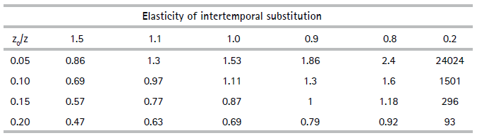
Note:For Colombia, value of elasticity of intertemporal substitution in benchmark is 0.16.
Source: author’s calculations.
For the interest rate we assume a value of 3% as reference, although the long-term cycles of interest rates and the cost of liquidity for families may vary substantially over time and within and across populations. Rates on government bonds have varied between the nineties and the first two decades of the millennium. In wealthier countries, real rates went from levels above 3% to near-zero or negative, while in emerging economies they went from near 10% to values not far from zero. Additionally, families rarely have access to the interest rates paid by government debt and may face steep charges for borrowing money. In wealthier countries financial markets offer lower costs of access to financing (including in the form of health insurance), while in other countries families usually find themselves in a range between no access to formal financing to expensive and constrained financing. For families, access to health insurance defines the interest rates that apply to the consumption of expensive health services, and lack of insurance often means that access to such procedures is closed.
The value of 8,766 hours available per year corresponds to 24 hours a day times 365.25 days; Murphy and Topel (2006) use a parameter of 4,000. A related issue is that the marginal value of leisure time is approximated with the salary. For workers, the argument relates to the analysis of the marginal decision to work longer hours, not the value of the time available to the person at other margins. How to value leisure time remains a pending issue. Aspects related to the home economy must be included in order to model the alternative margins, which are not only work and leisure, but also domestic work, sleep, and possibly others (Rosen, 1974).
3.2 Estimation of c, l, e, VLY and VSL
This section shows the estimates for equation 9 and explains the selection of the benchmark specifications, providing the data used to calculate VSLs. An Appendix details the results and is available from the author upon request.
In general, consumption follows a flag pattern (increases from childhood to early adulthood). Figure 1 shows consumption by age groups, standardized by the age group 30-49. Wealthier countries tend to have increases after prime ages, while other countries have flat or even declining profiles, as is the case of African countries. The causes may be benefits of the welfare state that promote consumption in old age and higher private savings in wealthier countries, and shorter life expectancies and lower qualities of life in old age that promote downward patterns in poorer countries. For example, the top left panel shows that compared with Canada and the United States, consumption in El Salvador is lower at older and younger ages, and is flatter over the lifecycle.
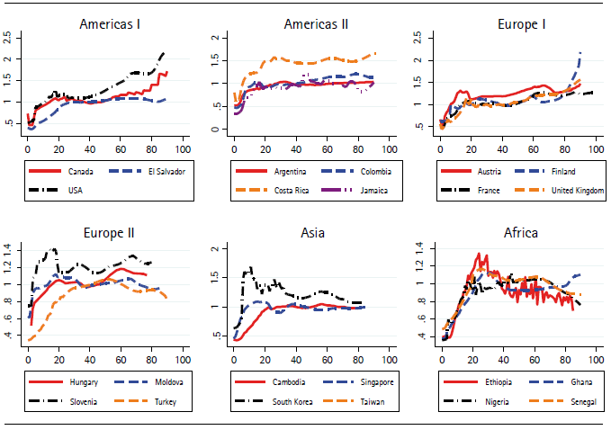
Source: author’s calculations using data from NTA (2019).
Figure 1 Consumption per capita by age relative to 30-49 age group
We chose the quartic model to construct the profiles of lifetime consumption. The quartic terms are significant only for the African region, but they seem to capture part of the difference in behavior between wealthier long-lived countries and poor short-lived countries. Figure 2 shows the predicted and actual values using the quartic models for four countries in the sample. We are evidently not capturing the upward trend that persists in wealthier countries after 80. On the other hand, data for those age groups is scarce and the weight for the population is low, so we do not expect our calculation of VLY to be affected very much. Many countries will reach life expectancies of above 80 during the present century, and the way savings, consumption, and labor will change will be a main issue for research, but something that we do not deal with here.
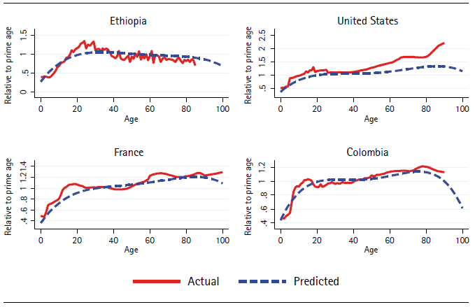
Source: author’s calculations using data from NTA (2019).
Figure 2 Actual and predicted consumption by age with regional slopes interacting with quartic age terms. Relative to 30-49 age group
Longer lifespans mechanically change the pattern of consumption, and the relation between wealth and consumption over the life cycle cannot be expected to be homogenous: expenditures on education, health entertainment, leisure, and other goods likely have a complex relation to wealth, and also involve marital behavior and other factors from which we must abstract. Human capital decisions affect health in complex ways as pointed out by McFadden (2008). Thus, the regression model is only an approximation to the pattern of consumption over the lifecycle within regions where countries face similar wealth and longevity constraints. The endogeneity of these patterns is certainly a major concern in this research.
In sum, we use the quartic model to predict the profile of consumption over the life cycle for all countries. We assign a regional profile to each country in the GBD sample following a simple regional criterion and multiplying the national consumption per capita by the profile to obtain consumption per capita by age.
To model leisure, we use data on labor force participation rates (Figure 3) and average hours of work in 2010 (Figure 4). Figure 5 shows the calculated average leisure hours. Leisure is a conventional term, but it is important to know that it does not mean unproductive time. Young individuals do not work mostly because they are investing in human capital, and older adults that retire can also invest time and a larger share of their income in healthier lifestyles. GDP per worker is the variable used to shift the level of the consumption and income profiles to monetary levels (/ in equation 10) and is shown in Figure 6. Figure 7 illustrates the profiles of labor income from the NTA database. Important surveys on the topic have been produced by Willis (1986), Card (1999), and Heckman, Lochner and Todd (2006). A key message is that a concave earnings pattern results mainly from school and on-the-job human capital decisions. We expect longevity to affect investment in human capital. Thus, longevity affects investments in human capital, generating potential biases in the estimation of VLY.
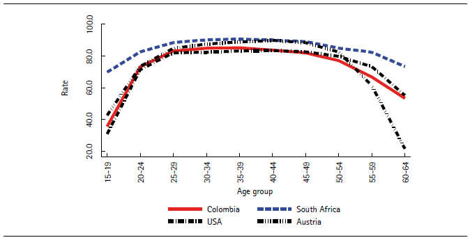
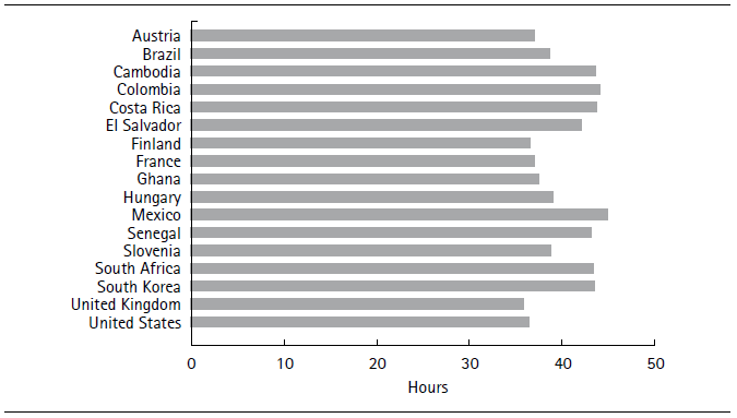
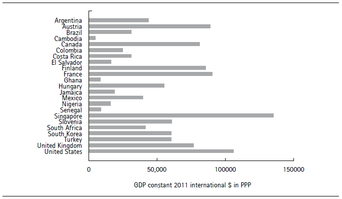
Figure 8 illustrates the results for some of the countries in the calculated model. The solid lines correspond to average observed labor earnings, and the dotted lines to predicted values. Projections are based on the cubic model (column c in Table 2).
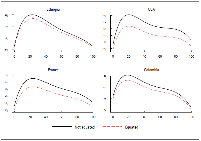
The present values of income and consumption are assumed to be equal across the life cycle. For each country, predicted consumption and income over life are  Equality means that a scalar α makes
  While no special meaning is assigned to α here, a concern is that measurement errors that determine the gap between average earnings and consumption correlate with longevity. In particular, the intergenerational transmission of wealth and capital income are likely higher in wealthier societies and can covary with health and longevity. Figure 8 shows the resulting profiles for a subsample of countries. The distance between the original consumption profile (these are predicted values from the regression model) and the profile that equates present values of consumption and income is positive in all cases, which means that true income is likely higher than the values reported by the variable we use. On the other hand, the distance is larger for wealthier countries, possibly due to higher capital income, which is not included in the variable we use to measure income. The consumption and income profiles are used to calculate full income and full consumption using data on amount of work. Figure 10 shows the results scaled to monetary units using GDP per worker.
Source: author’s calculations.
Figure 8 Age profiles of consumption with and without equating to value of income
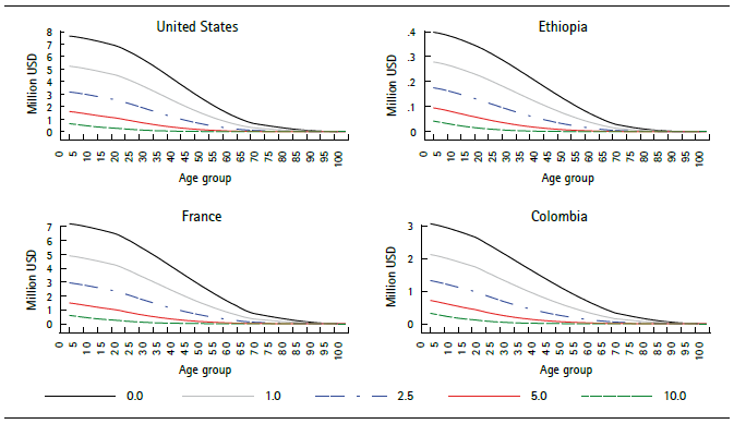
The discounted and non-discounted VSL for the benchmark case is shown in Figure 9. The remaining VSL by age is shown in Figure 10, which shows that wealthier countries have a much higher VSL. This does not mean that the lives of their citizens are more valuable, only that they are willing to pay more for improvements in longevity. Interest rates also have a large impact on the calculations for the remaining VSL, especially for children, due to the longer discount horizon (Figure 11). Under real rates above 2.5% that prevailed in the eighties and nineties, values for children are one half or less than those obtained at rates below 1%, which more closely reflect the reality of financial markets since 2008.
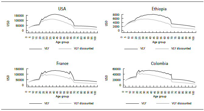
Source: author’s calculations using ILO data on participation (variable PR_MF); World Bank data on GDP per person employed (constant 2011 PPP $; variable sl_gdp_pcap_em_kd); and regression models for lifetime consumption and income. Parameters: sigma = 1.1; z0/z between 0.05 and 0.20 according to income; real discount rate = 0.01 per year.
Figure 9 Value and discounted value of life year by age in four countries
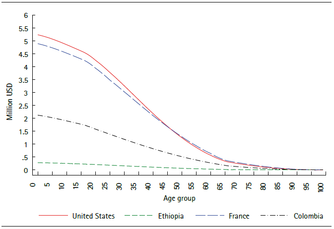
Source: author’s calculations.
Figure 10 Remaining Value of statistical life by age for four countries
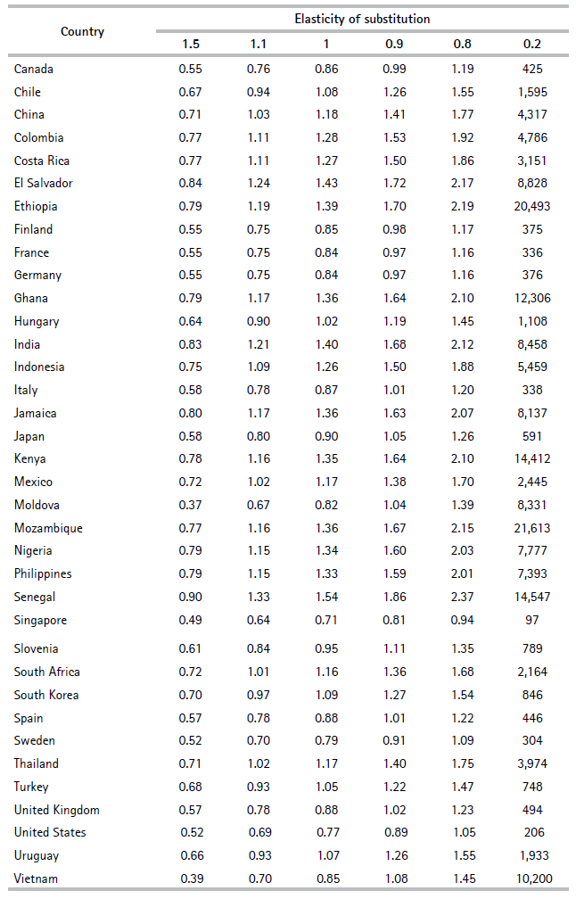
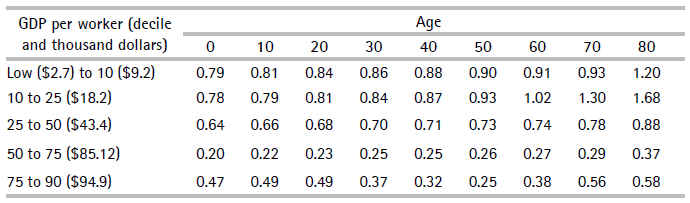
VLY estimates are higher when the elasticity of substitution is smaller (time provided by extra longevity is a more highly-valued good), and the ratio of GDP per worker to VLY is lower in wealthier countries; an extra year of life is worth only 75% of a year of productivity in Australia, but around 103% in Argentina and Brazil, and 133% in Senegal (Table 2, with σ = 1.1). Table 1 made an additional point: given a value of σ, the impact of being closer to subsistence consumption is significant, as shown in Table 3.
This section has described the data and calculations needed to obtain {y,c,l} for each country at each age, and shows calculations of v and VLY.
Table 2. Ratio of value of life year to GDP per worker to average for different values of elasticity of substitution
Source: author’s calculations.
4. Results, scenarios, and income elasticities
This section presents calculations of the value of improvements in health based on equation (8). The conceptual experiment is next: a small perturbation in survival probabilities is measured by ΔSa t, . If this perturbation is exogenous to full income and full consumption (namely, to labor force participation, income, and regional variables), then we can use the estimated values of Vt to calculate the value of an improvement in longevity.
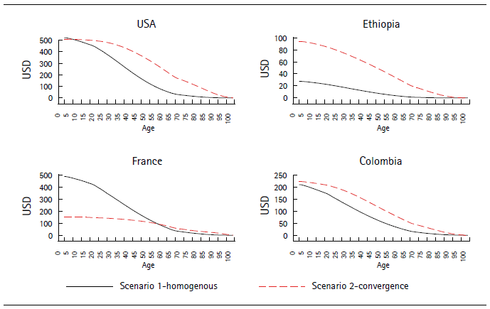
Scenario 1 assumes an improvement of 0.01% in survival probabilities across the whole lifetable of each country. This corresponds to the conventional measurement of VLY using 1 in 10,000 deaths as the decrease in risk. For Scenario 2, we use Singapore as a benchmark of longest-lived country, and the parameter δ= 0.0025 is chosen only to make the WTP roughly equal in both scenarios for middle income countries around the levels of Mexico and Colombia. Scenario 2 provides significant gains to the less healthy countries, and little to those with better survival profiles. For example, with this parameter, gains in survival probabilities for Colombia are in the order of 1 or 2 in 10,000 for children, around 5 at age 47, and 10 at 73. For Ethiopia, the figures are 6, 13 and 47 respectively, and for France they are 0.2, 1 and 4.
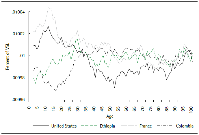
Figure 12 shows the VSL percentage gain in Scenario 1. Figure 13 shows the gains in money in Scenarios 1 and 2. For children, in Scenario 1, these range from around USD$500 for the wealthier countries to below USD$30 for the poorest. To provide some perspective consider this: in wealthy, middle-income and low-income countries infant mortality (death before first birthday) per 10,000 can be around 28 (France), 124 (Colombia) and 350 (Ethiopia). This highlights the challenge of incentivizing investment in health in countries with weak labor markets that offer very limited opportunities to families, as WTP for child mortality reductions can be very low in some countries.
For wealthier countries, percentage gains are greater for young age groups in Scenario 1 (homogenous improvements across life), which means that saving one additional life is very valuable there because the value of earnings and consumption is so high. In Scenario 2, percentage gains are higher for shorter-lived countries due to the way the counterfactual is constructed. In the convergence scenario, some countries (like the United States and Colombia) obtain most gains in middle age groups, some at older ages (France), and some at all ages due to their generally high mortality (Ethiopia).
Source: author’s calculations.
Figure 12 Percent gain in remaining VSL in Scenario 1 for four countries
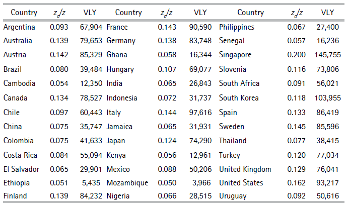
To calculate income elasticities of the remaining VSL, the percentage variation at each age is divided by the percentage change in the income variable between selected percentiles. In particular, the values correspond to percentiles 10, 25, 50, 75, and 90 (Table 4). Estimates are higher for lower income countries and for older ages, and in general are lower than one. Robinson, Hammitt, and O’Keefe (2019) recommend using values between 1.0 and 1.4 to extrapolate VSL calculated in wealthier countries to less developed countries for which no direct calculations are available. Their review of the practice in international organizations highlights that values below 1.0 are used to extrapolate calculations between more developed countries, and above 1.0 for the less developed. Our estimates contradict that practice and mean that our calculations of the remaining VSL yield higher values for lower income countries than in other studies.
Table 4 Income elasticities of remaining VSL by age at reference percentiles
Note:percentage change in remaining VSL divided by percentage change in GDP per worker. The percentage variation in income is calculated using as reference the 10, 25, 50, 75 and 90 percentiles of GDP per worker (for the first step, the lower reference point is the lowest value in the sample); corresponding levels in money are shown.
Source: author’s calculations.
The practice of transferring estimates from high to low-income populations is based on assumptions of income elasticities. In turn, the elasticities are obtained from datasets that combine information from studies conducted for different countries. Mardones and Riquelme (2018) follow the practice of relating estimates of VSL in previous studies to per capita GDP; they estimate a linear regression relating the logs of VSL (from published studies) to GDP per capita, and use values of the regressor for Latin American countries to obtain the values shown in the last column of Table 5. Those estimates have more variability than ours, determining very low values of VSL for some countries such as El Salvador. There are also differences due to the use of different income variables: GDP per capita or GDP per worker. The main issue is that the larger variability in VSL in the meta-analysis calculations produce higher income elasticities (low-income countries need to gain more in VSL per dollar of increase in income to reach the VSL levels of wealthier countries).
Table 5 Comparison with VSL calculated through meta-analysis
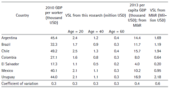
NoteThe first four columns correspond GDP per worker used in this study and to calculations of VSL at ages 20, 40, and 60, also in this research. The last two column are based on Mardones and Riquelme (2018).
Source: author’s calculations.
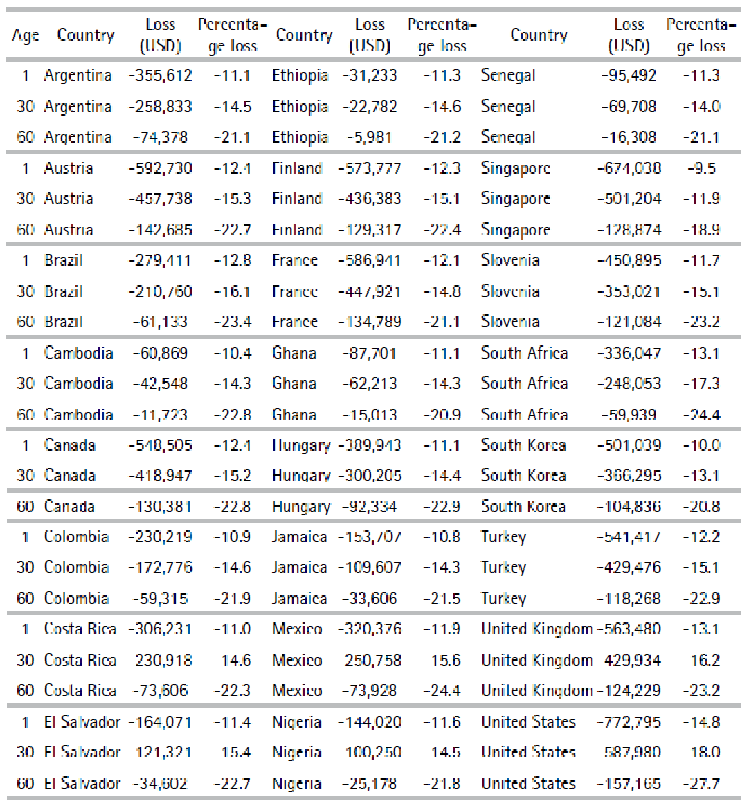
The role of disability is measured using data on Years Lost to Disability (IHME, 2017). The VLY is multiplied at each age by the variable H(t), which equals one minus the percentage rate of YLD and is an average of the time not spent on disability, weighted by the severity of disabilities in the population of each country. Sample values are around 0.96 and 0.98 for little children but are as low as 0.94 for Nigeria. At age 60, values hover around 0.8, but are 0.78 for the United States and 0.84 for Singapore. The interpretation of the level of this variable is ambiguous on welfare terms, especially at older ages. A longer-lived country could expect more disability under some circumstances. For example, a country where few healthy individuals reach old age (say, 70) will have a higher H-health value than a country with higher life expectancy where many reach the oldest age groups but including a mix with more less-healthy individuals.
Table 6 shows the effect of discounting for YLD on the calculation of VSL in the benchmark case. In money terms, for little children, the measured cost of expected disability over the remaining lifetime nears $772,795 in the United States and is barely above $31,000 in Ethiopia.
5. Prospects
The estimates of VSL presented here are unique because they are obtained directly from data that represent a wide class of countries, they consistently apply assumptions on the structure of preferences and its parameters, and provide a foundation for further research.
The main limitation of our estimates arises from the potential response of leisure and consumption to increased longevity and changing disability. The expected bias is not immediately discernable. On one hand, increased longevity lengthens the time available for work but, as in the basic labor supply model, income effects can induce lower levels of work. At more depth, the significant changes in longevity observed globally since at least the mid-20th century have produced major transformations in the family and the workplace. Individuals are also likely to make decisions on quantity and quality, as improved longevity increases the return on investments in human capital, such as healthy living and health prevention. Some of these changes may work towards reducing the value of GDP and other conventional measures of welfare because they involve tasks conducted in the home. Thus, time and cohort effects are likely relevant and, in the long term, work, consumption, and disability profiles are endogenous.
Other limitations come from data availability. Data on consumption by age group is the hardest to obtain, and besides the NTA project, we do not know of any other source. Data on labor variables is more common, but very few countries have extensive job market surveys. Finally, in terms of health, investment by the IHME provides a rich pool of national and subnational data to construct multi-year panels.
On the issue of the income elasticity of VSL, the conclusion is that values below 1 are the norm, and that values are smaller at higher wealth levels. Values below 1 are against the practice of using values above 1.0 to interpolate VSL values for lower income countries (i.e., values have been underestimated). Elasticities below 1.0 mean that the variability in VSL between countries is smaller than the variability in market income. This is consistent with the review by Doucouliagos, Stanley and Viscusi (2014) of valuations based on meta-analyses. The authors bias the values of income elasticities upward and after correcting, conclude that the income elasticity of VSL is “clearly and robustly inelastic.” This implies that the difference in VSL between wealthier and developing countries is smaller than what is implied by estimates based on meta-analyses.
The framework developed here can be used to calculate WTP for improvements in survival probabilities due to specific causes. Under the assumptions used, any change in S(t,a) can be evaluated. For example, a decrease in a specific cause in mortality, such as a type of cancer or Type II diabetes.
It is understood that the willingness to pay for reductions in risk can be studied in the framework of compensating variations (Thaler and Rosen, 1976). The ongoing COVID19 pandemic and the major adjustments taken by societies to contain the spread evince that individuals are willing to sacrifice substantial consumption resources to reduce the risk of death. A standard employed in this paper to measure the value of increased longevity is a gain of 1/10000 in risk, while the impact of COVID is already 10 times larger for many countries, and it probably will be 20 times larger by the end of 2021. A back of the envelope calculation (using Scenario 1), focusing on individuals aged 60, shows that in wealthier countries (Japan), individuals would pay around $1,100 to avoid the risk, $550 in middle income countries (Colombia), and $102 in a poor country (Cambodia). Nevertheless, societies face the usual challenge of setting prices and collecting revenues to supply public goods. This research deals with how much society is willing to pay for risk reductions, but not in terms of how to decrease a risk: willingness to pay does not equate a product’s availability on the market.

