Is historical VaR a reliable tool for relative risk measurement in the Colombian stock market?: an empirical analysis using the coefficient of variation*

Edgardo Cayón Fallon** Julio Sarmiento Sabogal***

* This article is one of the results of research project Number 1405, “Caracterización de los Metódos de valoración de Empresas en Colombia” 2002-2004, financed by the Pontificia Universidad Javeriana. Este artículo se recibió el 11-08-2003 y se aceptó el 27-05-2004.

** BS Economics and Finance, Syracuse University. 1995; MBA 2001 Mc Gill University. Assistant Professor, Management Department-FCEA Pontificia Universidad Javeriana. E-mail: ecayon@javeriana.edu.co.

*** Especialista en Gerencia Financiera de la Pontificia Universidad Javeriana, 2001; Administración de Empresas Pontificia Universidad Javeriana, 1998. Profesor, Departamento de Administración, Facultad de Ciencias Economicas y Administrativas, Pontificia Universidad Javeriana, Coordinador académico especialización en Gerencia Financiera, FCEA Pontificia Universidad Javeriana. E-mail: sarmien@javeriana.edu.co

ABSTRACT

Value-at-Risk (VaR) has become one of the most used techniques in financial risk management. The purpose of this paper is to address how well the technique holds in an illiquid stock environment, such as the one in the Colombian stock market. Our objective is to measure the efficiency of Value-at-Risk in terms of the coefficient of variation, which has been long used by practitioners, and treated frequently in the literature, as a measure of relative risk which is relatively easy to implement. Indeed, by using a simple regression analysis, we show how well VaR (specifically historical VaR) holds as a dependent variable, in terms of the coefficient of variation as our independent variable. The results fail to provide conclusive evidence that by CV standards, the historical VaR holds, on the average, as a reliable methodology for measuring risk at high confidence levels in the Colombian stock market. These results open another line of inquiry, if whether indeed the Colombian Stock Market behaves in a parametric or a non-parametric way, which could also put into question the effectiveness of the CV as a relative risk measure, a significant question that is a matter for further research that could lead to a whole different set of conclusions.

Key Words: Risk, Finance, Risk management, Quantitative Risk Analysis, stock market, Value at Risk

¿Es el VaR una herramienta confiable para medir el riesgo en el mercado de valores colombiano? Un análisis empírico mediante la utilización del coeficiente de variación

RESUMEN

El valor en riesgo se ha convertido en una de las técnicas más utilizadas en el manejo de riesgos financieros. El propósito de este artículo es mostrar cómo se comporta esta técnica en un entorno bursátil ilíquido, como el de la Bolsa de Valores de Colombia. Nuestro objetivo es medir la efectividad de esta técnica en términos del coeficiente de variación, la cual ha sido ampliamente usada por los expertos y mencionada con mucha frecuencia en la literatura, como una medición de riesgo relativo relativamente fácil de implementar. De hecho, mediante un análisis de regresión simple, se muestra que el valor en riesgo (especialmente el valor histórico) se comporta como una variable dependiente en relación con el coeficiente de variación, nuestra variable independiente. Los resultados no ofrecen evidencia contundente de que, según los estándares CV, el VaR histórico sea, en promedio, una metodología confiable para medir el riesgo con altos niveles de confiabilidad en el mercado de valores de Colombia. Los estudios abren otra línea de investigación sobre el interrogante de si dicho mercado se comporta de manera paramétrica o no paramétrica, hecho que también pondría en duda la efectividad del coeficiente de variación como técnica de medición del riesgo relativo. Esta pregunta amerita mayor investigación, la cual podría conducir a conclusiones totalmente diferentes.

Palabras clave: riesgo, finanzas, manejo del riesgo, análisis cuantitativo del riesgo, mercado de acciones, Valor en Riesgo.

Introduction

The concept of variance (commonly defined as standard deviation) as a measure of financial risk has been extensively treated in the financial literature. Most of the academic work surrounding variance as a potential risk measure is focused on Markowitz’s portfolio theory (Markowitz, 1952). Although no formal framework or general economic solution has been given to variance as a risk proxy in terms of economic utility, the intuitiveness behind variance as a basic statistical concept makes it easy to use (Brief and Owen, 1969). Indeed, most of the theoretical work about this subject is concerned with seeking rules in the context of “probability beliefs” for the “rational investor”, rather than seeking a solution for one size fits all (Markowitz, 1991). The basic premise of this “set of rules” is that most investors tend to be risk adverse (defined in statistical variance¹ terms), and will be just barely willing to accept more variance (or higher risk), if and only if this risk is compensated for in terms of a higher expected return (defined in terms of the historical statistical mean² ). Under this basic premise, we define the coefficient of variation and VaR (specifically historical VaR) as standard measures of risk.

Definitions

The coefficient of variation is defined mathematically as:

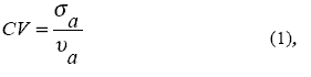
where ^σ_a is defined as the standard deviation of X observations of the stock or asset a, and ^υ_a is defined as the expected return of X observations of the stock or asset a. This definition is often used as a measure of relative risk, and should be used for comparison purposes among different investment choices. However, it is important to recall that this is a measure that always has to be compared relative to another investment; otherwise it is completely useless. For illustration purposes, let’s use the following data for Stocks A and B:

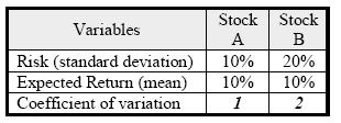
As we can see, there is not much use in knowing that the CV for stock A is 1, but when compared to the CV for stock B of 2, we can infer that this stock is twice as risky as stock A. The measure is straightforward in the sense that the higher the CV of one stock or asset as compared to another, the riskier that stock is in terms of variance (measured by the standard deviation). In other words, the CV can measure the dispersion of two different data series from their respective expected returns, and therefore their relative risk.

Although the CV is commonly used in investment analysis, there has been a debate concerning the instances in which it should be applied to investments. When used in the estimation of risk premiums among a certain number of data series, it has been found that when a certain degree of autocorrelation exits among the variables combined in a portfolio, the high variance variables tend to be underestimated, due to the covariance effect in the portfolio as a whole (Scheel, 1978). Furthermore, when measuring the CV of stand-alone investments, such as stocks, we have to assume that the expected return is the ratio of two random variables³ (Brief and Owen, 1969). Besides the randomness prerequisite, also the data series of the stock should be parametric (normally distributed); in the case of nonparametric data (not normally distributed), the appropriateness of the CV as a relative risk measure can be put into question (Dewitt and Roberts, 1970). However, there is strong theoretical and empirical evidence that supports the fact that stocks tend to distribute normally and behave in a random manner. As the theoretical basis, (Samuelson, 1965) provided a mathematical proof via stochastic processes as to why it is impossible to predict future stock prices based on historical data, and as to why they will behave randomly under a specified set of assumptions. This notion is further reinforced by an empirical study conducted by Eugene Fama; this study, which comprised 30 highly traded stocks form the NYSE, showed evidence that stocks tend to behave as a random walk and as independent events (Fama, 1965). This notion of independence is pivotal in proving that stocks are indeed normally distributed. Therefore, we can conclude that the CV can be a good measure of relative risk, when applied to stocks.

In the early 1980s, Value-at-Risk (VaR) was implemented by major US banks as a methodology for measuring market risk in absolute (monetary) terms. The use of this methodology was further reinforced by the Basle Committee on Banking Supervision, due to the negative impact of the major international financial crisis of the 1990s to the world’s major financial institutions (Jorion, 2002). VaR is a very simple measure, easy to understand, and can be defined as the predicted worst-case loss at a specific confidence level (e.g. 95%) over a certain period of time (e.g., 1 day).⁴ In other words, VaR measures risk in terms of the worst-case past occurrences to the left of a normal distribution tail, given a specified probability range. This is done with the purpose of finding the observation that represents the exact percentage loss for that specific probability range. Although there are many methodologies for VaR calculation, in the specific case of the Colombian stock market, we will use the most common and easy to implement, which is historical VaR.⁵ For the purpose of measuring the Historical VaR of a single asset (each of the selected Colombian stocks), we have to do the following calculations:

· Obtain a historical price dataset for the asset in question.

· Calculate the historical returns of each observation, using the following formula:

Where P ₀ = next day s price

P₁ = previous day s price

· Then the resulting series of historical returns should be arranged in ascending numerical order (e.g. –0.02%,-0.01%, 1%, etc.)

· To determine which point in the series will give us the exact VaR at a specific confidence level, we use the following formula:

Specific point in the historical series = n_X X n

Where n_X=(1-α)

 α = the given confidence level (e.g. 95%)

n_X = the percentile outside the given confidence level (e.g. 5%)

n = total number of historical observations

· Finally, multiply the % value that corresponds to the specific point in the series by the monetary value invested in the asset, and that gives us our VaR for that specific confidence level (It is always important to keep in mind that VaR has to be expressed as a monetary loss; e.g., Col$ -37.000).

As we can see, historical VaR has an intuitive appeal on the grounds that it provides a range of possible losses on ongoing investments. Therefore, it gives the investor an easy-to-understand criterion for investment selection on the grounds of risk aversion (expressed in absolute monetary terms). It also provides a criterion that solves some of the paradoxes⁶ involved in investment selection based solely on the grounds of expected return and risk as is intended in portfolio theory. On the other hand, it gives risk managers a day-to-day tool to determine the tendency of risky investments, and to what extent this can have a monetary impact on the investment portfolio as a whole.

Nevertheless, we believe that historical VaR has some validity as an effective risk measure, due to the fact that it relies on the historically observed, worst-case past scenarios. We want to test the reliability of the measure, when compared to another risk measure with equal intuitive and even better theoretical appeal, such as the CV. Since both the CV and the historical VaR tend to denote higher amounts of risk, the higher the result is, then our question is straightforward: Is Historical VaR an efficient tool for risk measure in the Colombian stock market?

In order to answer this question and test the efficiency of the historical VaR in the Colombian stock market, we will run a simple regression, where the CV of a series of Colombian stocks will act as the independent variable and the historical VaR of those stocks as our dependent variable. If indeed historical VaR is a good measure of risk (because a higher CV should denote a higher historical VaR based on the reasons stated before), then we will reject our null hypothesis that there is no relation at all between the two risk measures, by using the p-value as a measure for determining the significance of the regression.

1. The Dataset

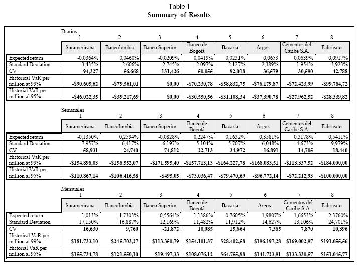
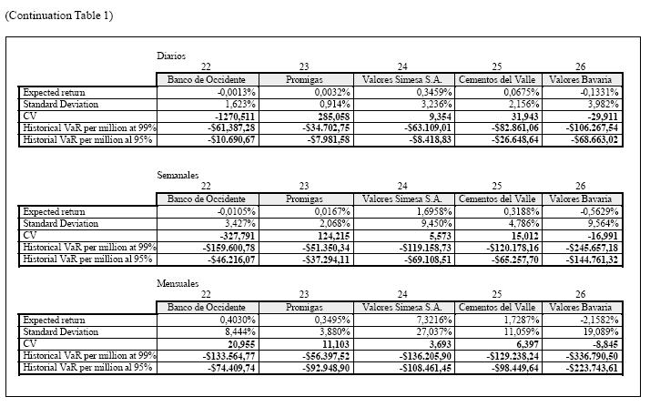
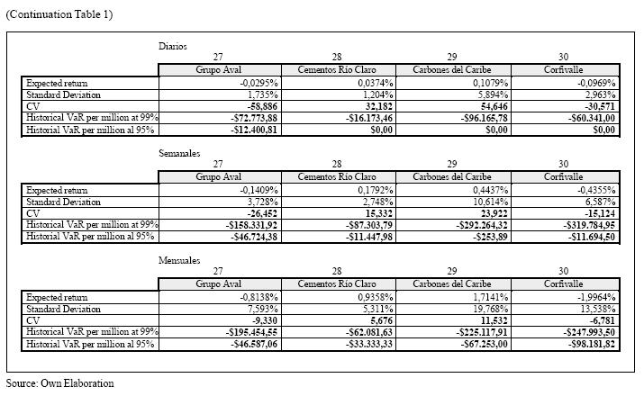
The dataset is comprised of 30 Colombian stocks and their daily average trading price from the year 1998 to 2003. Due to the small size of the Colombian Stock market, just half of these stocks are actually traded on a daily basis,⁷ therefore making the Colombian stock market an illiquid stock environment in liquidity terms. On the average, we have 1354 daily observations⁸ per stock, this being the range of observations between 1454 and 536 on a daily basis, 288 weekly observations on average, this being the range of observations between 310 and 113 on a weekly basis, and 66 monthly observations on average, this being the range of observations between 72 and 26.⁹ In order to test our hypothesis, we chose the three different holding periods¹⁰ in order to compute both the CV an the historical VaR. The frequency of the holding periods for each stock was daily, weekly and monthly.¹¹ Since the historical VaR has to be given in absolute terms, we chose a preset amount of Col$ 1,000,000 per stock, thus giving a standard measure of historical VaR per million investment in each stock.¹² Table 1 summarizes the results we found for each stock on a daily, weekly and monthly basis. For the historical VaR calculation, we chose the 95% and 99% confidence levels, respectively.¹³

Table 1

Table 1A

Table 1B

Table 1C

2. Testing the hypothesis

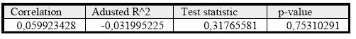
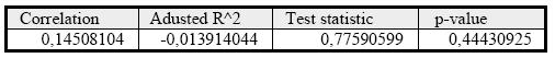
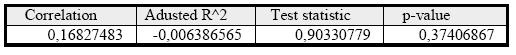
As mentioned before, we ran a total of six regressions, using CV as our independent variable and historical VaR at different confidence levels as our dependent variable. In order to test our hypothesis of linearity,¹⁴ in which a higher CV denotes a higher historical VaR, we have to reject our null hypothesis that there is no linear relationship between the two variables using p-value.¹⁵ The p-value is straightforward; if the p-value (which is set at α = 0.05 and α = 0.01 for 95% and 99% confidence intervals respectively) is higher than our critical value for p, then there is a linear relationship between the two variables. Otherwise, we fail to reject our hypothesis -and accept the null hypothesis that there is no linear relationship at all between the two variables. The regression results are as the follows:¹⁶

2.1 Computed daily CV as the independent variable and daily historical VaR at the 99% confidence level as the dependent variable (summary of results df=28¹⁷)

H₀: There is no linear relationship between the daily CV and the historical daily VaR at the 99% confidence level.

H₁: There is a linear relationship between daily CV and the historical daily VaR at the 99% confidence level.

P-Test: We fail to reject the null hypothesis and have to accept that there is no evidence that a linear relationship exists between the daily CV and the historical daily VaR at the 99% confidence level.

2.2 Computed daily CV as the independent variable and daily historical VaR at the 95% confidence level as the dependent variable (summary of results df=28)

H₀: There is no linear relationship between the daily CV and the historical daily VaR at the 95% confidence level.

H₁: There is a linear relationship between daily CV and the historical daily VaR at the 95% confidence level.

P-Test: We fail to reject the null hypothesis and have to accept that there is no evidence that a linear relationship exists between the daily CV and the historical daily VaR at the 95% confidence level.

2.3 Computed weekly CV as the independent variable and weekly historical VaR at the 99% confidence level as the dependent variable (summary of results df=28)

H₀: There is no linear relationship between the weekly CV and the historical weekly VaR at the 99% confidence level.

H₁: There is a linear relationship between the daily CV and the historical weekly VaR at the 99% confidence level.

P-Test: We fail to reject the null hypothesis and have to accept that there is no evidence that a linear relationship exists between the weekly CV and the historical weekly VaR at the 99% confidence level.

2.4 Computed weekly CV as the independent variable and weekly historical VaR at the 95% confidence level as the dependent variable (summary of results df=28)

H₀: There is no linear relationship between the weekly CV and the historical weekly VaR at the 95% confidence level.

H₁: There is a linear relationship between weekly CV and the historical weekly VaR at the 95% confidence level.

P-Test: We fail to reject the null hypothesis and have to accept that there is no evidence that a linear relationship exists between the weekly CV and the historical weekly VaR at the 95% confidence level.

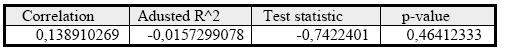
2.5 Computed monthly CV as the independent variable and monthly historical VaR at the 95% confidence level as the dependent variable (summary of results df=28)

H₀: There is no linear relationship between the monthly CV and the historical monthly VaR at the 95% confidence level.

H₁: There is a linear relationship between monthly CV and the historical monthly VaR at the 95% confidence level.

P-Test: We fail to reject the null hypothesis and have to accept that there is no evidence that a linear relationship exists between the monthly CV and the historical monthly VaR at the 95% confidence level.

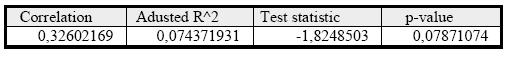
2.6 Computed monthly CV as the independent variable and monthly historical VaR at the 90% confidence level as the dependent variable (summary of results df=28)

H₀: There is no linear relationship between the monthly CV and the historical monthly VaR at the 90% confidence level.

H₁: There is a linear relationship between monthly CV and the historical monthly VaR at the 90% confidence level.

P-Test: We fail to reject the null hypothesis and have to accept that there is no evidence that a linear relationship exists between the monthly CV and the historical monthly VaR at the 90% confidence level.

We fail to reject six out of six of our null hypotheses, and we have to accept that there is no evidence that there is a linear relationship between the CV and the historical VaR for different holding periods and high confidence levels.

3. Concluding Remarks

By assuming that the coefficient of variation is a reasonably accepted methodology for measuring relative risk, both in practice and in theory, we fail to provide conclusive evidence that by CV standards, the historical VaR holds, on average, as a reliable methodology for measuring risk at high confidence levels in the Colombian stock market. Although we fail to reject the null hypothesis in all the cases, this fact can be explained by the fact that there are not enough historical monthly observations to make our result statistically sound,¹⁸ which can also distort the results obtained at certain confidence levels.¹⁹ This opens another line of inquiry; that is, whether, the Colombian Stock Market behaves in a parametric or a non-parametric way, which could also put into question the effectiveness of the CV as a relative risk measure, a significant question that is a matter for further research that could lead to a whole different set of conclusions. For the time being, we cannot prove in a conclusive manner that historical VaR is indeed a reliable risk measure in a thinly traded environment such as the Colombian Stock Market.

Footnotes

1. For the mathematical formula of variance (defined as standard deviation), see Appendix A .

2. For the mathematical expression of expected return (defined as historical mean), see Appendix A .

3. Usually in the comparison of stand-alone investments, the expected return (and therefore standard deviation) is done on a one-period basis, since the prices (historical) are known and not random. The problem arises for the future expectations in a multi-period basis, since the incorporation of future (unknown) observations makes it impossible to compute the actual mean and variance for that future, and consequently the true actual return; this is why it is called “expected return”, since the chance of being equal to the actual return is random.

4. Riskmetrics Group. (1999).

5. As is implemented by RiskmetricsTM.

6. For a better understanding of this issue, please refer to Baumol (1963).

7. For further information concerning how the stocks are ranked in terms of trading and other methodological issues on the reliability of the available public data, please go to the following website http://www.supervalores.gov.co/

8. In Colombia we use the weighted average daily price methodology. This methodology disguises the effect of dividends on the price of the stock.

9. In the specific cases of Colombiana de Inversiones S.A. and Valores Simesa S.A., the stocks were initially registered on October 10, 2001 and June 16, 2001 respectively.

10. A holding period for our purposes is defined as the investment horizon for buying and selling each stock (i.e., if I buy today and sell tomorrow, my holding period was daily; if I buy today and sell at the end of the week my holding period was weekly, etc.)

11. These are the most commonly used holding periods for computing VaR; for further discussion, please see Riskmetrics-Technical Document.

12. For simplicity purposes, we assume that there are no transaction costs involved, due to the fact that these costs tend to vary enormously on the basis of the trading frequency of each stock.

13. This confidence level applies for daily and weekly only. For the monthly VaR, the confidence level is set at 95% and 90%, due to the fact that there are not enough observations for a higher confidence level.

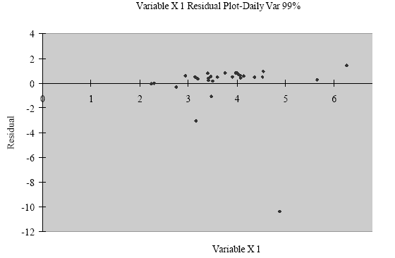
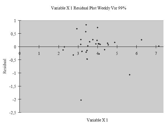
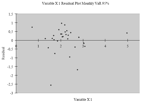
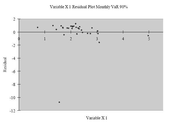
14. Due to the fact that the computed numbers can present the problem of heteroscedasticity, the previous dataset is expressed in absolute terms, and then logarithmically transformed for variance stabilizing purposes. Even with the logarithmic transformation, the residual plots (Appendix B) show strong evidence of a non-linear relation between the variables. In the case of negative CVs, we use absolute values because of the symmetric characteristic of this measure (a negative CV denotes a negative expected return or the possibility of making a short sell, but its relative risk is the same).

15. When we calculate the p-value, we are calculating the probability of obtaining a value of the test statistic (which is recommended for small samples as in this case) more extreme than the one we actually have; since we have both positive and negative values, our p-value is computed on a two-tail basis.

16. A negative adjusted R^2 denotes that the X variable cannot explain the Y variable and also serves as a test of multicollinearity.

17. Degrees of freedom.

18. At least 60 historical observations are recommended to make it statistically significant.

19. This is reinforced by the fact that there are not enough observations to calculate the historical VaR at the 99% confidence level for certain stocks (see Table 1).

Bibliographical References

Aczel, A. D. Complete Business Statistics, Boston (MA), Irwin. 1993.        [ Links ]

Baumol, W. J. “An Expected Gain-Confidence Limit Criterion for Portfolio Selection”, in: Management Science, 1963. v. 10, n. 1, October.         [ Links ]

Brief, R. P. and Owen, J.. “A Note on Earnings Risk and the Coefficient of Variation”, in: Journal of Finance, American Finance Association, 1969 v. 24, December, pp. 901-904.         [ Links ]

DeWitt, R.; Roberts, C., and Roberts, E. N. “Exact Determination of Earnings Risk by the Coefficient of Variation”, in: Journal of Finance, American Finance Association, v. 25, 1970. December, pp. 1161-1165.         [ Links ]

Fama, E. “The Behavior of Stock-Market Prices”, in: Journal of Finance, American Finance Association, 1965. v. 38, March, pp. 34-105.         [ Links ]

Jorion, P. Value-at-Risk. New York: McGraw Hill. 2002.        [ Links ]

Markowtiz, H. “Portfolio Selection” in: Journal of Finance, American Finance Association, 1952. v. 7, March, pp. 77-91.        [ Links ]

“Foundations of Portfolio Theory” in: Journal of Finance, American Finance Association, 1991.v. 46, June, pp. 469-477.         [ Links ]

RiskMetrics Group. Risk Management. A practical guide. New York. 1999.        [ Links ]

Risk Metrics-Technical Document. New York: JP Morgan/Reuters. 1996.        [ Links ]

Scheel, W. C. “Comparison of Riskiness as Measured by the Coefficient of Variation”, in: The Journal of Risk and Insurance, American Risk and Insurance Association, 1978.v. 45, March, pp. 148-152.         [ Links ]

Samuelson, P. A. “Proof that Properly Anticipated prices Fluctuate Randomly”, in: Industrial Management Review, MIT Press, 1965. V.6, Spring pp. 41-50         [ Links ]

Data Source

http://www.supervalores.gov.co

Appendix A

Standard deviation is defined as:

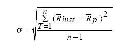
Donde: R_hist.= Historical observations expressed in returns terms.

R_p.= Historical expected return

n = Number of observations.

Expected return is defined as:

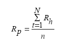
R_p = Expected Return

R_h = Historical Return

n = number of observations

Appendix B-Summary of Residual Plots