^* This article is a research paper based on the project Risk and Return in Latin American Financial Markets. Beginning: January 1, 2007. Ending: December 31, 2008. This project was funded by ICESI University, Cali, Colombia. The article was received on 07-06-2009 and was accepted for publication on 28-10-2009.

^** Economista, Universidad ICESI, Cali, Colombia, 2006. Correo electrónico: marcos@icesi.edu.co

^*** PhD in Business, Tulane University, New Orleans, USA, 2005; Master in Management, Tulane University, 2001; Especialista en Administración, Universidad ICESI, Cali, Colombia, 1997; Especialista en Finanzas, Universidad ICESI, 1996; Ingeniero eléctrico, Universidad de los Andes, Bogotá, Colombia, 1987. Jefe del Departamento de Finanzas, Universidad ICESI. Correo electrónico: jbenavid@icesi.edu.co

^****Doctor en Administración de Empresas con énfasis en Finanzas, Tulane University, New Orleans, USA; Master in International Finance, University of Amsterdam, Amsterdam, Holanda; Especialista en Finanzas, Universidad ICESI, Cali, Colombia; Economista, Universidad del Valle, Cali, Colombia. Profesor de tiempo completo, Departamento de Finanzas, Univesidad ICESI. Correo electrónico: lberggru@icesi.edu.co.

ABSTRACT

This article uses four methods to derive optimal portfolios comprising investments in the seven most representative stock exchanges in Latin America from 2001 to 2006 and it studies their composition and stability through time. The first method uses a historical variance - covariance matrix and the second one employs a semi-variance -semi-covariance matrix. The third method consists of an exponentially weighted moving average and the fourth and last method applies resampling. From a practical point of view, this result is significant because less rebalancing can mean greater potential savings. The article further analyzes the performance of optimal portfolios as compared to equally weighted portfolios. The results of applying the Sharpe ratio in the out-of-sample period provided no evidence of statistically significant differences between optimal portfolios and equally weighted portfolios. However, some evidence is provided in favor of resampling as the returns obtained in the out-of-sample period showed stochastic dominance over the returns of the portfolios estimated using more traditional methodologies.

Key words: Optimal portfolios, portfolio resampling, stochastic dominance, Latin America.

RESUMEN

Este documento utiliza cuatro métodos para derivar portafolios óptimos con inversiones en los siete mercados accionarios más representativos de Latinoamérica y estudia su composición y estabilidad temporal. El primero usa una matriz de varianza y covarianza histórica; el segundo, una matriz de semivarianza y semicovarianza; el tercero, un promedio móvil con ponderaciones exponenciales, y el último, remuestreo. Desde una perspectiva práctica, este resultado es importante, pues los ahorros por un menor rebalanceo pueden ser considerables. Además, se comparó el desempeño de estos portafolios óptimos ante portafolios equitativamente diversificados. No se hallaron diferencias estadísticamente significativas en la razón de Sharpe de portafolios optimizados y portafolios equitativamente diversificados en el período fuera de muestra; sin embargo, hay evidencia a favor del remuestreo, por cuanto los retornos obtenidos en este período presentaron dominancia estocástica sobre los retornos de portafolios estimados con metodologías más tradicionales.

Palabras clave: portafolios óptimos, remuestreo de portafolios, dominancia estocástica, Latinoamérica.

RESUMO

Este documento utiliza quatro métodos para derivar portfólios ótimos com investimentos nos sete mercados de ações mais representativos da América Latina e estuda sua composição e estabilidade temporária. O primeiro usa uma matriz de variância e covariância histórica; o segundo, uma matriz de semi-variância e semi-covariância; o terceiro, uma média móvel com ponderações exponenciais, e o último, reamostragem. Desde uma perspectiva prática, este resultado é importante, pois a economia com um menor reajuste pode ser considerável. Além disso, comparou-se o desempenho destes portfólios ótimos com portfólios equitativamente diversificados. Não se encontraram diferenças estatisticamente significativas na razão de Sharpe de portfólios otimizados e portfólios equitativamente diversificados no período fora da mostra; entretanto, tem-se alguma evidência a favor da reamostragem, quanto aos retornos obtidos neste período apresentaram dominância estocástica sobre os retornos de portfólios estimados com metodologias mais tradicionais.

Palavras chave: portfólios ótimos, reamostragem de portfólios, dominância estocástica, América Latina.

Introduction

Markowitz (1952) is considered the forefather of modern investment theory. He proposed that the problem of selecting an optimal portfolio should only be considered in terms of the mean and variance of asset returns.

More specifically, Markowitz showed that the problem could be simplified as one of finding the portfolio that maximized returns at any given of variance or, equivalently, finding the portfolio that minimized variance returns at some level of portfolio returns. If he can solve this optimization problem, the investor can find the efficient frontier that shows different combinations of risk and return obtained with efficient portfolios that include only risk assets. Admitting to some degree of risk aversion, this investor can choose a utility maximizing portfolio.

When there is a risk-free asset in the market, it is easy to show that the optimal portfolio that includes only risky assets is independent of an investor's risk aversion. This is usually known as the separation theorem (or property, see Tobin 1958). One of the implications of this theorem is that the problem of choosing an optimal portfolio can be thought of as finding a tangency portfolio to a ray emanating from the y-axis (risk free return) to the efficient frontier in the standard deviation-return plane. In this way the tangency portfolio will maximize the ratio of expected return (in excess of the risk free rate) to standard deviation (Sharpe ratio).

Several authors have recognized practical shortcomings when trying to apply Markowitz methodology. The literature has stressed the difficulties in estimating expected returns and covariances and the impact of changing assumptions about these optimization inputs in resulting portfolio weights. Moreover, the optimization eventually suggests portfolio weights that tend to be concentrated in a few assets and are prone to change abruptly when the optimization is effected in a different, albeit close, period.

For instance, Green and Hollifield (1992) recognize lack of diversification in optimal portfolio weights as a serious shortcoming in Markowitz optimization. More specifically, they note that as the number of assets grows, portfolio weights constructed from sample moments, do not approach to zero and sometimes involve extreme positions. The paper goes to study the question if mean variance efficient portfolios and "well-diversified" portfolios concur. The characteristics of these "well- diversified portfolios" are connected to bounds on the means of portfolio returns in terms of their average absolute covariance with the individual assets.

Black and Litterman (1992) acknowledge two problems that plague optimal portfolio allocation exercises. The first one is the difficulty in measuring expected returns and the second, the high sensitivity of allocation of results to return assumptions. They propose a model that merges both Markowitz methodology and Black's (1972) version of the CAPM to derive equilibrium risk premiums and consequently portfolio composition that tilt toward equilibrium values (i.e. portfolio weights are stationary and respond to an investor's views of relative performance across assets).

Britten Jones (1999) derives (artificial OLS) t-tests and F-tests for inference on tangency portfolio weights and linear restrictions on these weights. The idea is to find the portfolio closest to an arbitrage portfolio (unitary excess returns and zero standard deviation). This portfolio is the usual tangency portfolio and its composition can be found by an (artificial) OLS regression. Empirically, the paper studies the magnitude of sampling errors of efficient portfolio weights for an American investor for the period (1977-1996). Across three different sub-periods changes in portfolio (country) composition are considerable as well as the standard errors of portfolio weights¹. Moreover, the author is unable to reject the null hypothesis that diversification brings no benefits for an American investor in the period².

More closely related to this paper, Michaud (1998) has identified instability and ambiguity as the two major weaknesses of Markowitz traditional approach. Changes in optimization inputs (standard deviations, expected returns and covariances between assets) can lead to significant changes in the optimal portfolio composition in terms of both cross-section and time-series. Consequently portfolio optimality is not clearly defined. Michaud provides a framework³ in which the optimization problem can be thought of in a statistical way, in which portfolio weights are subject to estimation error and through simulation these weights can be included in (familiar) confidence intervals and be subject to hypothesis testing.

The purpose of this paper is to study the varying composition of optimal (tangency) portfolios of risk assets derived following several approaches. Tangency portfolios comprise US dollar investments in the seven most important stock markets in Latin America (Argentina, Brazil, Chile, Colombia, Mexico, Peru and Venezuela) from September 2001 to December 2006.

Furthermore, it studies the stability of these portfolio weights and tries to determine if there is a tendency of these weights to revert to mean values. In addition, this document analyzes the performance in terms of risk and return of these optimal portfolios and compares it to that of an equally-weighted portfolio (naïve diversification).

The paper finds that the use of "traditional" methods to forecast variances and covariances of asset returns (historical variances-covariances and historical semivariances and semicovariances) and to derive the optimal portfolio composition, suggested portfolio compositions rather similar interms of cross-section and in time-series. The optimal portfolio composition is time varying and presents abrupt changes that may seriously impede practical application. The optimal portfolio weights do not show symptoms of mean reversion and sometimes these weights involve extreme positions in some countries that may prove unbearable to many investors.

Using Michaud's method, we found more stable (not necessarily stationary) portfolio weights, weights that are dissimilar to those obtained by more "traditional" methods as well as more diversified (less concentrated) portfolios that may benefit an investor by substantially reducing transaction costs and in some cases (as we find in Section 4) provide some gains in terms of risk-adjusted returns. Moreover, diversification can bring some benefits in terms of risk reduction.

The rest of the document is organized as follows: the second section deals with the estimation of the tangency portfolio both in presence and absence of a risk-free asset and explores four methods of obtaining portfolio weights of the tangency portfolio. These methods are closely related to different approaches to estimate the variance covariance matrix; a key input in the optimization process. The third section presents further details of the data and empirical methodology used to study the composition, stability and performance of these optimal portfolios. The fourth section discusses the results and finally the fifth section includes some concluding remarks.

1. Tangency portfolio composition

In order to calculate the composition of the optimal or tangency portfolio (T) we will initially consider the case where there is no riskfree asset and where short selling is allowed⁴. This analysis can be easily modified to allow for the existence of a risk-free asset. An investor with some degree of risk aversion will choose a portfolio that maximizes the ration ^r _σ; where r and σ stand for the mean and standard deviation of returns.

Figure 1 depicts the hyperbola (efficient frontier) showing risk and return combinations of these optimal portfolios. The line emanating from the origin that touches the efficient frontier in point T (or tangency portfolio) shows different risk return combinations of portfolios comprising investments in risk assets as well as in a zero return zero standard deviation asset⁵. In this sense, portfolio T represents a 100% investment in a risk portfolio.

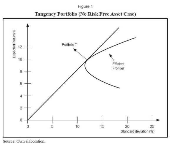
The problem of finding the optimal portfolio is related, then, to finding the composition of portfolio T, the one that maximizes the slope of the line emanating from the origin.

Before stating the problem in matrix terms, it is necessary to remember that the expected return of a portfolio can be calculated as w^Tr and that the variance in portfolio returns will be given by w^TVw, where r and w represent column vectors (n×1) of expected returns and weights respectively, T stands for transpose, n represents the number of assets in the portfolio and V stands for the variance covariance matrix.

To facilitate calculations it is possible to work with the function log . The Lagranbian will be:

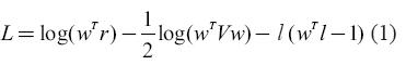
The objective function is then to maximize the return-risk ratio under the restriction that the sum of portfolio weights will be equal to one⁶. After some matrix operations (see Ingersoll, 1987), we obtain an expression to estimate the composition (w) of the tangency portfolio:

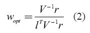
When there is a risk free asset the optimization problem slightly changes. In this case the optimal portfolio will be given by:

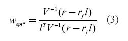
r_f stands for the risk free rate. The reader will notice that equations (2 and 3) critically depend on an estimate of the variance covariance matrix of asset returns. Naturally, these equations also require an estimate of expected returns. In this paper the sample mean will serve as such estimate, though we recognize the existence of other methods to forecast expected returns and the potential problems involved with this approach (see Black and Litterman, 1992).

As previously mentioned, this document will explore the effects of different estimations of the variance covariance matrix that update in time (V_t), in the composition of optimal portfolios comprising investments in Latin American stock indexes denominated in dollars. In this regard, this paper takes the perspective of a U.S. or dollar denominated investor that wishes to build an optimal portfolio with stock investments in the most important markets of Latin America. The four methods used to estimate the variance covariance matrix and derive the tangency portfolio are:

1.1 Historical variance covariance matrix⁷

This is perhaps the most common way of estimating the variance covariance matrix of stock returns. The sample variance of returns will be given by:

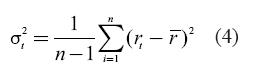
Where r^-) represents the expected return in the sample and n stands for the number of observations. The reader will notice that this method assigns the same weight to returns both below and above the mean to measure risk. In addition, this method allocates the same weight to the n observations used to calculate variances in the return. The sample covariance will be equal to:

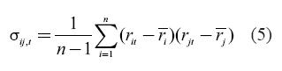
Covariance measures the co-movement between two series (i and j). As in the case of the variance, this estimation considers equally both the returns below and above the mean and gives the same weight to all observations in the sample used to estimate this measure of co-movement.

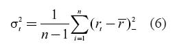
1.2 Semivariance semicovariance matrix

This method, very similar to the previous one, considers only the periods when the returns are below the mean to estimate the variance of returns:

The covariance of returns will be given by the following expression:

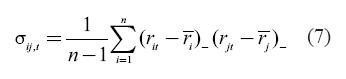
Where (r_it − r_i )₋ represents returns below the mean for asset i in time t. Bear in mind that in the sum only the days (or time periods) when returns are below the mean are included.

1.3 Exponentially Weighted Moving Average (EWMA)

The previous methods gave the same weight to all observations, while this method assigns weights differently for each observation and as such, it gives more weight to more recent observations.

This method to estimate volatility was initially proposed by JP Morgan under the trademark RiskMetrics^®. By and large, the variance in time t will be:

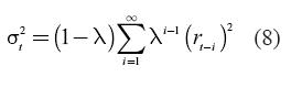
In this case λ is also called a decaying factor, and it is less than one. In particular, JP Morgan sets λ equal to 0.94 for daily data and 0.97 for monthly data. From the previous equation it is easy to derive:

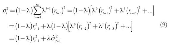
In short, the current period variance will be equal to λ times the volatility in the previous period plus (1 – l) times the previous period square return. The expression of the covariance will be:

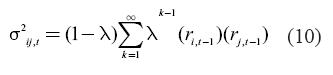
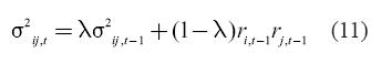
Solving recursively for the covariance, we get:

1.4 Estimating the tangency portfolio through resampling

The previous three methods and perhaps other more traditional methods suffer from what is usually known as sampling error. Due to the fact that optimization results tend to over-weight assets with high recent returns (leaving aside reversion to the mean features of asset returns) and with low covariances and correlations that do not necessarily hold during the investment period. In this setting, suggested portfolio weights can change abruptly in time causing optimization results to be impractical or counter-intuitive. Furthermore, the changes in portfolio composition (in time) can demand high transaction costs thus making traditional portfolio optimization an expensive proposition. All these issues have been recognized in the previous literature (Green and Hollifield, 1992; Black and Litterman, 1992; Britten-Jones, 1999).

This fourth method allows quantifying the impact of sampling error using the related concept of portfolio resampling. It should be remembered that the parameters (r and V) used in the optimization exercise are just a possible realization of asset returns history. In other words, if a different sample is used, the portfolio weights suggested by the optimization will be different. The portfolio resampling technique is a way to confront this randomness in the optimization inputs.

To do this, it is initially assumed that it is possible to estimate the optimization parameters with the available sample of returns and denote these parameters as r₀ and V_0* With these initial parameters it is feasible to construct an initial efficient frontier (or "original").

Then, by using bootstrapping techniques or parametric techniques, such as random sampling from a multivariate normal distribution of returns during N times, it is possible to obtain a series of parameters V₁,r₁,..., V_N,r_N. With these different vectors of expected returns and variance covariance matrices it is possible to find the composition of N tangency portfolios (as well as N efficient frontiers).

These tangency portfolios (with their weight vectors w₁,...,w_N) are then plugged in using the original sample of returns that was used to get r₀ and V₀ in order to estimate the risk and return characteristics of the resampled portfolios (e.g. w^Tr and w^TVw). As a consequence, the tangency portfolios will lie below the "original" efficient frontier; in other words, these portfolios are inferior in term of riskreturn characteristics since the weight vectors were estimated with error⁸. The further the points from the initial efficient frontier the more acute the problem of sampling error.

In this section we illustrate the methodology proposed by Michaud (1998) which uses similar simulation techniques as previously described that mitigate sampling error and allow retrieving the composition of the tangency portfolio.

This method requires initially an estimate of V_t (i.e. an historical approach). Then, the portfolios of minimum risk (Q) and maximum return (R) in the efficient frontier are identified. Next, the method requires analyzing a series of points equally distant (in terms of returns) that lie in the efficient frontier between Q and R. In this study, we used 500 points or portfolios on the efficient frontier.

A random sample of returns is then obtained (i.e., assuming that returns follow a multivariate normal distribution) and this permits an estimate to be made of the vector of expected returns and V. This new vector and new matrix are used to repeat the optimization exercise and hence produce a new efficient frontier.

This simulation procedure is repeated a significant number of times, thus obtaining a large number of efficient frontiers. Then at each level of returns between Q and R, weights suggested by the different optimizations are averaged and subsequently a new "average" or re-sampled efficient frontier is constructed. Finally, with this re-sampled efficient frontier we find the tangency portfolio as the one that maximizes the return to risk ratio.

2. Methodology

This section discusses in depth the estimation of the dynamic tangency portfolio constructed with the use of investments in stock indexes of seven Latin American countries.

2.1 Data

Return series were estimated using MSCI price indices in US dollars from Datastream of the stock markets of Argentina, Brazil, Chile, Colombia, Mexico, Peru and Venezuela for the period September 1999 to December, 2006 for a total of 382 weekly observations. We used as the risk-free rate the 3-month Treasury Bill rate (secondary market) reported by the Federal Reserve.

A weekly frequency was used to estimate the dynamic tangency portfolios since it reflects a reasonable compromise between the high costs of daily portfolio rebalancing and the relatively limited information when monthly returns are chosen. Table 1 shows some descriptive statistics of the weekly⁹ logarithmic returns for the whole sample.

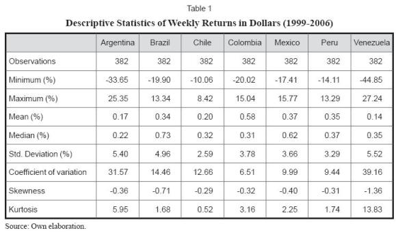
The table shows that the Colombian stock market reported the highest average return in the period while the Venezuelan stock market the lowest. These results are partially explained by the relative strengthening of the Colombian peso and the weakening of the Venezuelan Bolívar versus the dollar during the sample period.

Venezuela and Argentina were the most volatile markets during the period whereas the stock markets in Chile and Peru were the most stable ones. Colombia, Peru and Mexico showed the lowest coefficient of variation in country returns pointing to more stable markets when adjusting for the magnitude of mean returns. Latin American stock indices presented slightly negative skewness. Kurtosis was more pronounced in returns for the Argentinean and Venezuelan markets.

In a dominance analysis, Argentina dominated Venezuela since it had higher mean returns and lower risk (standard deviation). Brazil, as well as Chile, dominated Argentina and Venezuela. Colombia, Mexico and Peru dominated (each) Argentina, Brazil and Venezuela. Moreover, according to this analysis, Venezuela did not dominate any country in the period and Chile was clearly not dominated by the three best-performing countries in the whole period (Colombia, Mexico and Peru).

In short, Colombia, Mexico and Peru dominated the largest number of countries in the sample (3) and Venezuela and Argentina had the worst performance in terms of dominance. Perhaps Chile and Brazil are "in- between" markets that dominated the two weakest markets. However, Chile showed a much lower risk as well as a lower coefficient of variation than Brazil (in fact, Chile had the four lowest coefficient of variation among the seven countries in the sample).

2.2 Estimation of dynamic tangency portfolios

Following equations (2) and (3) to ind the composition of the optimal portfolio and the four different methods to estimate the tangency portfolio, we used a rolling window technique to obtain different values of V_t and r_tand consequently different estimates in time of the optimal portfolio weights that update as new information (regarding returns and covariances of Latin American markets) arrives.

The fixed size of the estimation window was 104 weeks (2 years) and thus 174 estimations of the optimal weights were obtained beginning in September 2001 and finishing in December, 2004¹⁰.

2.3 Performance analysis in the out-of-sample period

Considering that one of the purposes of this paper is to analyze the efficacy in terms of risk and returns of efficient (optimized) portfolios, an out-of-sample analysis was conducted using the last two years of the sample (2005 and 2006). More specifically, this section analyzes what would have been the return and risk for an investor rebalancing its portfolio according to the optimal weights suggested by the optimization exercise. Additionally, this section compares the performance of these optimized portfolios to that of an equally weighted portfolio.

The statistic proposed by Jobson and Korkie (1981) was used to analyze whether significant statistical differences in portfolio performance of optimized versus an equally weighted portfolio were attainable in the out-of-sample period, This statistic tries to measure whether there are any statistically- significant differences in the Sharpe ratios of two portfolios, say i and j. More specifically, the null and alternative hypotheses of the test are:

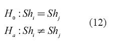
Jobson and Korkie (JK) proposed the following statistic:

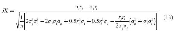
This statistic follows a standard normal distribution. In this case, we constructed portfolio pairs where portfolio i was fixed as the equally weighted portfolio and portfolio j as the optimized portfolio (in the presence of a risk free asset).

In addition, we conducted a second order stochastic dominance analysis for the return series in the out-of-sample period (2005-2006). According to this criterion, portfolio i will stochastically dominate portfolio j if:

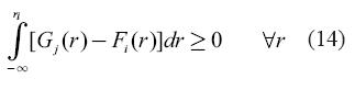
G and F represent the cumulative distribution functions (CDF) of portfolio j and i returns respectively. By using the cumulative distribution function of return this more comprehensive analysis not only incorporates means and variances of returns as in classical (financial) optimization theory but also other moments of the return distribution.

This means that if i dominatesj, the cumulative area below the CDF of j must be larger than the cumulative area for i. Second order stochastic dominance can be more readily understood in the context of two assets having the same mean, in which case the asset with the lowest variance will be the dominant one. In this section, we formed pairs for returns obtained using the different approaches to estimate the tangency (and equally weighted) portfolios for the out-of-sample period.

2.4 Stationarity tests on the time series of optimal weights per country

Because the previous analysis allows us to construct seven time series (weekly frequency) of portfolio weights for the countries in the sample, we conducted stationarity tests on these series of optimal weights to check whether there are mean reversion effects in the composition of optimal Latin American stock portfolios.

From a practical point of view, the existence of stationarity in one of the series would imply, for instance, a smaller need to rebalance the portfolio with respect to a particular country investment. The aforementioned, since one can expect short-term variations in the portfolio weight allocated to a certain country, but in the long run, this portfolio weight would exhibit a tendency to return to its mean value.

The tests used here are usually known as Augmented Dickey-Fuller and Kwiatkowski et al. (KPSS) tests. Taking into account the large changes in the weights for a particular country in the out-of-sample period, we decided to exclude the periods where the optimization exercise suggested consecutive 0 or 100% weights for a country index.

3. Results

In this section we analyze the changing portfolio composition in the presence of a risk-free asset and short-selling restrictions (weights constrained between 0 and 1) for the in sample period (September 2001 - December 2004) and out-of-sample period (2005-2006). For the latter period we also analyzed the performance and stationarity of country composition of tangency portfolios.

3.1 Tangency portfolio composition in the in-sample period

Tables 2a and 2b shows a series of descriptive statistics related to the mean and coefficient of variation of the optimal portfolio weights in the tangency portfolios estimated according to different approaches.

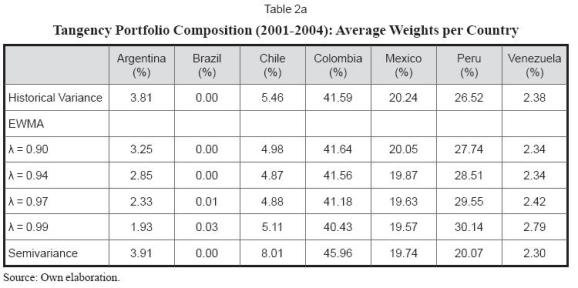
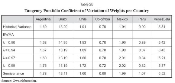
These methods suggest, on average, similar portfolio compositions tilted to investments in Colombia, Peru and Mexico that comprise roughly 85% of the tangency portfolio. The rest of the portfolio would be invested in Chile, Argentina and Venezuela. The optimization exercise suggested a null investment in the Brazilian market.

By and large, this analysis concurs with the dominance analysis of section 2.1, which showed better performance by the dominant (country) components in the tangency portfolio. The only exception is Brazil which, a bit surprisingly, does not enter the tangency portfolio. Perhaps this country's high risk as well as elevated coefficient of variation and negative skewness can explain this result.

It can also be seen that portfolio weights' coefficient of variation is especially high for the case of Venezuela. In relative terms the less volatile weights (according to their coefficient of variation) refer to investments in Colombia, Peru and Argentina.

For reference, figures 2a and 2b shows the changing portfolio composition when using an historical variance covariance approach. By and large, this varying portfolio composition can be related to our dynamic (or rolling) optimization that causes expected returns and variance covariance matrices to change in each optimization period. The horizontal axis shows dates (week number) in which the tangency portfolio was calculated and the vertical axis shows portfolio weights in the optimal portfolio (for the seven countries these weights add up to one in any given week).

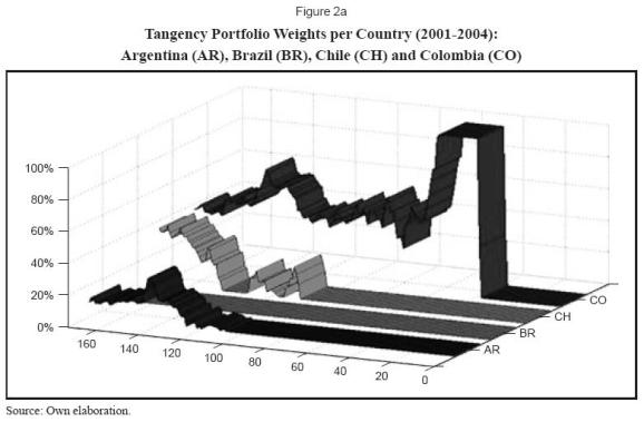
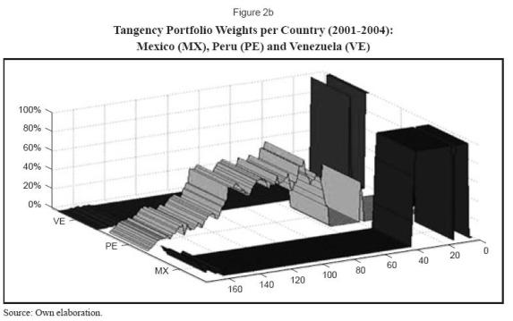
For the first year (September 2001 - September 2002), the tangency portfolio was completely invested in Mexico and then in Colombia. Peru, Colombia and Chile represent the whole tangency portfolio in the following two years and during this period Chile considerably increases its share in the tangency portfolio as well as Mexico (to a lesser extent), replacing investments in Peru.

Analyzing the Colombian case, the portfolio weight allocated to this country started to decline by the end of 2002 and it reached a 40% share of the portfolio by the end of 2004.

The case of Argentina case is interesting since the portfolio weights coincide with an improvement of the economic situation of the country. For most of the period, the portfolio allocation to that country was null and began to be non-zero almost two years after September, 2001. From then onwards (last quarter of 2003), Argentina's share averaged 10% of the tangency portfolio. The economic situation of the country improved¹¹ around that period, long after the economic disarray the country experienced from late 2001 to early 2002.

From a more general perspective these results highlight two weaknesses often cited in the classical optimization literature. These two weaknesses refer to the existence of undiversified portfolios; many investors would consider weights of more than 40% allocated to a particular country (or asset) excessive, and of sudden shifts in portfolio compositions that inhibit many portfolio managers to use the results suggested by the optimization exercise in practice. These shifts are more prevalent in the beginning of the period.

3.2 Tangency portfolio composition in the out-of-sample period

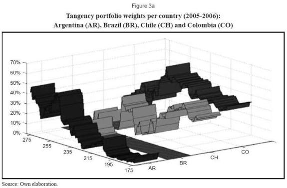
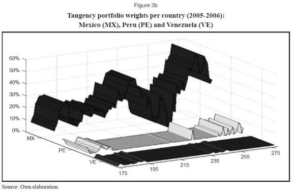
Tables 3a and 3b shows average weights per country for the tangency portfolio in this period. The tangency portfolio is concentrated in investments in Colombia, Mexico and Chile and then followed by investments in Argentina, Peru and Brazil. Venezuela's share in the tangency was practically nonexistent over the period.

The tables shows initially significant differences in average weights per country obtained in this out-of-sample period and the previous analyzed in sample period. Moreover, the table shows significant differences in portfolios weights attained thorough more traditional methods when compared to the resampling portfolio technique. This latter approach suggests a more diversified portfolio (less extreme investments in high and low weight markets, for instance, Brazil and Venezuela). For illustration, figures 3a and 3b shows the changing portfolio composition when using an historical variance covariance approach.

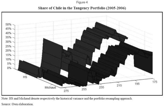
Further, the optimization exercise suggested some important timing differences in portfolio allocation by country and by estimation method (see Figure 4). This figure shows the differences in allocation between the historical variance and portfolio resampling approach for the particular case of Chile. Most notably, the highest difference in allocation in the period was an astonishing 30% and the lowest difference totaled 13%. Differences between the two methods averaged 3.5%.

The Table 3b shows a measure of weight dispersion that points to the fact that the semivariance approach tended to suggest more volatile weights (see the case of Argentina, Colombia, México and Peru) while the resampling portfolio approach tended to suggest less volatile or more stable weights per country.

Altogether, the two characteristics of resampling present in our sample (stability and diversification) can be very attractive for a portfolio manager since they add practical value to the optimization exercise and entail significant transaction cost savings since the need for portfolio rebalancing decreases.

3.3 Stationarity tests results of the time series of optimal weights per country

Unit root tests shown in tables 4a and 4b allow us to conclude that the time series of optimal weights have a degree of integration equal to one, except for the case of Brazil and Venezuela. In other words, theses tests show that for some countries their optimal weights will be subject to rebalancing without a clear trend to converge or return to the mean weight. For the specific case of Brazil and Venezuela, the optimal portfolio weights for these two countries fluctuated around minimum and maximum values and thus these tests do not provide conclusive evidence of the degree of integration of the series.

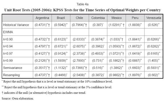
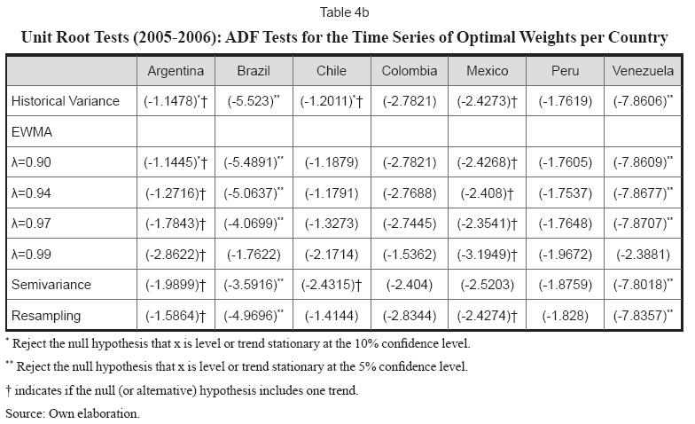
In summary, even though the previous section provided evidence that the optimal portfolio weights obtained through portfolio resampling techniques were more stable and less volatile, this does not necessarily mean that the optimal portfolio weights have to be stationary or mean reverting.

3.4 Performance analysis in the out-of-sample period

Table 5 shows some descriptive statistics of the mean and standard deviation of returns for the different portfolios during the out-of sample period.

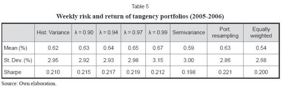
As it can be seen from the previous table, the equally weighted portfolio (or naïve diversification) showed the lowest average return as well as the lowest risk in the period. The most profitable and the riskiest portfolio was obtained through the exponentially weighted moving average method with a decaying factor equal to 0.99. The optimal portfolio estimated following Michaud (1998) attained the best return -standard deviation ratio (or Sharpe ratio) and the portfolio using an exponentially weighted moving average with a decay factor equal to 0.97 obtained the second best Sharpe ratio.

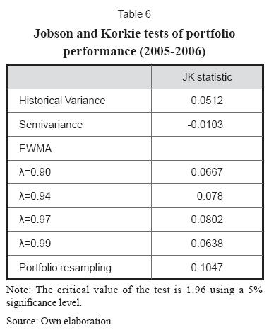
We used the test proposed by Jobson and Korkie (1981) to test if the differences in portfolio's Sharpe ratios were significant. This test compares the Sharpe ratio of an equally weighted portfolio to that of optimized portfolios. The low values of the statistic (see Table 6) allows to conclude that during the period there were no significant differences in mean -variance performance between optimized and equally weighted portfolios.

A second order stochastic dominance test was conducted to further our performance analysis for different pairs of portfolio combinations. This analysis is perhaps more general than that addressed by Jobson and Korkie (1981) since it incorporates all the moments of a portfolio return distribution. The results of the stochastic dominance tests are summarized in Table 7.

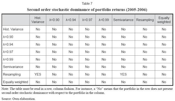
For most of the combinations (portfolio pairs) there is no evidence of second order stochastic dominance. Furthermore, optimized portfolios do not stochastically dominate a naïve equally weighted portfolio. However, the optimal portfolio obtained through resampling stochastically-dominated portfolios using the historical variance covariance matrix and the semivariance semicovariance matrix, thus providing some evidence for this particular sample of the benefits of resampling when deriving efficient portfolios. These results coincide with those of Jorion (1992) and Chopra, Hensel and Turner (1993) who found that portfolios constructed with simulation performed better than classical optimization portfolios in an out-of-sample window.

These results can be useful for researchers and portfolio managers when trying to forecast expected returns and covariances in emerging markets and more specifically to those managers facing the problem of investing in emerging markets analyzed in Goetzmann and Jorion (1999) and in our particular case, the problem of investing in Latin American markets that eventually will be “discovered” by foreign investors (e.g. Ecuador)¹².

Conclusions

This paper analyzed the composition of dynamic tangency portfolios invested in the stock indices of the seven most representative stock markets in Latin America both for an in-sample period (September 2001 - December 2004) and an out-of-sample period (2005-2006).

An historical variance covariance matrix, a semivariance semicovariance matrix, an exponentially- weighted moving average to estimate variance and covariance terms as well as portfolio resampling techniques were used to derive the composition of these dynamic tangency portfolios.

By and large, optimal weights suggested by the first three methods were quite similar whereas the weights suggested by portfolio resampling were more stable (not necessarily stationary). This last technique allowed a higher degree of diversification (minimizing extreme positions in both high and low weight stock markets). These two characteristics of resampling (stability and diversification) can be very attractive for a portfolio manager since they add practical value to the optimization exercise and entail significant transaction cost savings, since the need for portfolio rebalancing decreases.

Regarding portfolio performance during the out-of-sample period, the results point to no superior performance of optimized versus equally weighted portfolios (naïve diversification). However, the results when measuring performance using a second order stochastic dominance criterion provide some evidence in favor of resampled portfolios (Michaud, 1998) in lieu of portfolios using more conventional optimization techniques (historical variance covariance matrix and the semivariance semicovariance matrix).

A possible extension of this paper would be to work with multivariate GARCH models to obtain forecasts of the variance covariance matrix and thus of optimal portfolios weights and then compare the time stability and performance of these tangency portfolios to that of the portfolios analyzed in this paper. An additional extension would be to work with alternative utility functions -by assumption we worked with a quadratic utility function as in Markowitz (1952)- such as an exponential utility function that is frequently used in more recent literature related to portfolio optimization¹³. This would allow further analysis of the differential impact of using resampling instead of more traditional techniques in obtaining optimal portfolios.

Finally, another possible extension would be to examine the influence of stock market and economic development indicators of the countries in the sample (such as stock market capitalization to GDP, GDP growth or investment growth) in the tangency portfolio composition using regression analysis. The issue is whether country allocations in the tangency portfolio are better explained by relative economic and financial development or just by currency considerations (appreciation or depreciation of Latin American currencies vis a vis the dollar). An economic impact analysis would allow disentangling which of the two effects is stronger in explaining allocations across countries.

Footnotes

1. For instance, for Belgium the mean weight in the tangency portfolio during 1977-1996 was 29% with a standard error of 35.1%. During the 1977-1986 period the mean portfolio weight for that country was only 7.1% with an standard error of 46.8%.

2. In other words, the null hypothesis stating that the weights in the optimal portfolio of all foreign countries (Australia, Austria, Belgium, Canada, Denmark, France, Germany, Italy, Japan and the U.K.) are jointly zero was not rejected.

3. Nobel laureate Harry Markowitz informally conceded that Michaud’s methodology in regards to attaining efficient frontiers and optimal portfolios was superior to his. For details, see Chernoff (2003).

4. This analysis is different from that in Black (1972).

5. In the more realistic case of the existence of a risk free asset in the market the line starts at the level of the risk free rate (not at the origin).

6. l stands for a column vector (n×1) of ones.

7. This and the next two subsections are based on Alonso and Berggrun (2008).

8. The tangency portfolios (1,..., N) will not be efficient if they are evaluated using the initial data since by construction, the tangency portfolio obtained thorough the "original" efficient frontier is the most efficient portfolio (it is possible to denominate this portfolio as tangency portfolio 0).

9. The weekly returns were calculated from a series containing daily data (Friday to Friday).

10. Due to the high computational cost (more than 85 million simulations) required to apply Michaud's (1998) method in a rolling fashion, in this section we only calculated the time series of portfolio weights for the first three methods discussed in section 2.

11. This improvement was sustained for the following 3 years when the country GDP's grew by more than 8%.

12. Goetzmann et al. (1999) show that historically markets 'emerge' and 'submerge' due to internal crises, wars, communism or because investor lack of interest in a particular market. According to the paper, submerged markets can be understood as those that did not exceed USD 1 billion market capitalization threshold and the IFC no longer collected data on these markets. Emerging markets, on the contrary, are those markets that relatively recently exceeded that threshhold and are subject to data collection of international bodies. In this regard, Ecuador can be considered as a submerged market since some data collecting agencies do not record historical prices in this market (for example, MSCI indices for the Ecuadorian stock market are non-existent).

The paper shows that current 'emerging' markets have quite a long history (for instance, the Colombian stock market was founded in 1929 but the IFC only covered this market since 1984).The authors show that returns after emergence are quite different and much higher than those before emergence. Consequently, if investment decisions are based on recent returns (postemerging or in any way extrapolating using only the most recent available data) this can lead to unsatisfactory results. The case of Argentina is illustrative. The average yearly dollar returns in that country was 57.9% after emerging, while in the pre-emerging ('submerged') period was -18.2%.

Portfolio resampling, along with other techniques such as value at risk and scenario analysis, can mitigate this problem by giving a lower weight to the most recent data and thus being more conservative in allocating portfolio weights to markets that recently have had exuberant returns.

13. Markowitz optimization only takes into account the mean and variance of returns. Other utility functions that take into account different moments of returns distribution can add value in a portfolio optimization exercise. In addition, the assumption of a quadratic utility function has been criticized since a utility function of this type entails both an increasing absolute and relative risk aversion.

References

1. Alonso, C. J. and Berggrun, L. (2008). Introducción al análisis de riesgo financiero (1^st ed.). Cali: Editorial Universidad ICESI.         [ Links ]

2. Black, F. (1972). Capital market equilibrium with restricted borrowing. Journal of Business, 45 (3), 444-455.         [ Links ]

3. Litterman, R. (1992). Global portfolio optimization. Financial Analysts Journal, 48 (5), 28-43.         [ Links ]

4. Britten-Jones, M. (1999). The sampling error in estimates of mean-variance efficient portfolio weights. Journal of Finance, 54(2), 655-671.         [ Links ]

5. Chernoff, J. (2003). Markowitz says Michaud has built a better mousetrap. Pensions & Investments, 31(26), 3-39.         [ Links ]

6. Chopra, V. K.; Hensel, C. R. and Turner, A. L. (1993). Massaging mean-variance inputs: Returns from alternative global investment strategies in the 1980s. Management Science, 39 (7), 845-855.         [ Links ]

7. Cosset, J.-C. and Suret, J.-M. (1995). Political risk and the benefits of international portfolio diversification. Journal of International Business Studies, 26 (2), 301-318.         [ Links ]

8. Goetzmann, W. N. and Jorion, P. (1999). Re-Emerging Markets. Journal of Financial & Quantitative Analysis, 34 (1), 1-32.         [ Links ]

9. Green, R. C. and Hollifield, B. (1992). When will mean-variance efficient portfolios be well diversified? Journal of Finance, 47(5), 1785-1809.         [ Links ]

10. Ingersoll, J. E. (1987). Theory of financial decision making. Totowa, N.J.: Rowman & Littlefield.         [ Links ]

11. Jobson, J. D., & Korkie, B. M. (1981). Performance hypothesis testing with the sharpe and treynor measures. Journal of Finance, 36 (4), 889-908.         [ Links ]

12. Jorion, P. (1992). Portfolio optimization in practice. Financial Analysts Journal, 48 (1), 68.         [ Links ]

13. Kwiatkowski, D.; Phillips, P. C. B.; Schmidt, P. and Shin, Y. (1992). Testing the null hypothesis of stationarity against the alternative of a unit root: How sure are we that economic time series have a unit root? Journal of Econometrics, 54 (1-3), 159-178.         [ Links ]

14. Markowitz, H. (1952). Portfolio selection. Journal of Finance, 7 (1), 77-91.         [ Links ]

15. Michaud, R. O. (1998). Efficient asset management: a practical guide to stock portfolio optimization and asset allocation. Boston: Harvard Business School Press.         [ Links ]

16. Morgan, J. P. (1996). RiskMetrics technical document (4^th ed.). New York: Author.         [ Links ]

17. Scherer, B. (2002). Portfolio resampling: Review and critique. Financial Analysts Journal, 58 (6), 98-109.         [ Links ]

18. Tobin, J. (1958). Liquidity preference as behavior towards risk. The Review of Economic Studies, 25 (2), 65-86.         [ Links ]