^* This paper is one of the results of finance research projects financed by CESA and PUJ. This paper is a detailed and refined example of how to value callable bonds in emerging markets using real market data. This example is based in great part in the methodological approach developed by Salomon Brothers as explained in Fernando Rubio, Valuation of Callable Bonds: The Salomon Brothers Approach (July 2005). The article was received on 13-05-2008 and was accepted for publication on 28-10-2009.

^** MBA, McGill University, Montreal, Canadá, 2001; BS Economics and Finance, Syracuse University, New York, United States, 1995. Profesor asociado en Finanzas, Colegio de Estudios Superiores de Administración (CESA). E-mail: ecayon@cesa.edu.co.

^*** Especialista en Gerencia Financiera, Pontificia Universidad Javeriana, Bogota, Colombia, 2001; Administrador de empresas, Pontificia Universidad Javeriana, 1998. Profesor, Departamento de Administración, Facultad de Ciencias Económicas y Administrativa, Pontificia Universidad Javeriana. Coordinador académico, especialización en Gerencia Financiera, FCEA, Pontificia Universidad Javeriana. E-mail: sarmien@javeriana.edu.co.

ABSTRACT

This article aims to shed light on the issues that stock brokers face upon implementing the binomial model when valuating corporate bonds with a multiple exercise option for the issuer. To that end, the proposed methodology is used to valuate this type of instrument in the company Transportadora de Gas del Interior Internacional Ltda. (TGI). In the specific case of TGI, it was found that the binomial model enables finding the value of the spread points that can be attributed to the option and that, employing that measure, the sole risk measure attributable to a specific corporate activity can be obtained.

Key words: valuation, callable bonds, OAS, emerging markets.

RESUMEN

El propósito del artículo es clarificar algunos de los problemas que los profesionales de la bolsa encuentran al implementar el modelo binomial en la valoración de bonos corporativos con opciones de ejercicio múltiple por parte del emisor. Para ello se propone una metodología que valora este tipo de instrumentos, utilizando los bonos de la Transportadora de Gas del Interior Internacional Ltda. (TGI). En el caso específico de la TGI se encontró que empleando el modelo binomial es posible hallar el valor de los puntos de spread atribuibles a la opción, y con esta medida también obtener una medida del riesgo único atribuible a una actividad corporativa específica.

Palabras clave: valoración, bonos redimibles, OAS, mercados emergentes.

RESUMO

O propósito do artigo é esclarecer alguns dos problemas que os profissionais da bolsa encontram ao implementar o modelo binomial na valoração de bônus corporativos com opções de exercício múltiplo por parte do Banco Central. Para isso propõe-se uma metodologia que valoriza este tipo de instrumentos, utilizando os bônus da Transportadora de Gás do Interior Internacional Ltda. (TGI). No caso específico da TGI encontrou-se que empregando o modelo binomial é possível descobrir o valor dos pontos de spread atribuíveis à opção, e com esta medida obter também uma medida do risco único atribuível a uma atividade corporativa específica.

Palavras chave: valoração, bônus corporativos, OAS, mercados emergentes.

Introduction

Unlike the pricing of equities, and setting the issue of credit quality aside, the pricing of bonds depends solely on the future behavior of interest rates and their effect in discounting future expected cash flows. Where bonds have embedded calls from the issuer, this represents a distinct challenge, because the issuer can alter the nature of the cash flows that the investor will receive depending on the future behavior of interest rates.

Therefore, given the fact that the issuer can recall the bond at his convenience, the investor faces a substantial risk of prepayment from the part of the issuer. This characteristic can often be detrimental to the investor, because usually the issuer will recall the bond at a higher discount rate than that which can be obtained in the open market, thus generating a loss to the investor who is forced to sell the bond back to the issuer at a price below the real market value of the bond at the future time of the transaction (Rubio, 2005). Since the investor faces the risk of an uncertain stream of cash flows, the common market practice is to demand a higher yield in a callable bond than in a non-callable bond in order to compensate the higher risk caused by the embedded call options in a specific issue.

In common practice, the credit and liquidity risk of any common non-callable bond is determined by the additional yield spread paid by that bond when compared to the yield of a risk-free bond with a similar maturity date (i.e. Corporate Issues vs. U.S. Treasuries). In the case of callable bonds the additional spread demanded by the investor over and above the credit and liquidity risk premium is known as the Option Adjusted Spread (OAS). In order to calculate the OAS, assumptions have to be made about the behavior of the uncertainty of the stream of cash flows of the bonds and their effect on future yields, and therefore modeling risk is a factor that has to be taken into account when valuing callable bonds (Henderson, 2003). In the US numerous studies have been conducted regarding the behavior of the OAS of callable vs. non-callable bonds. For example, Longstaff (1992) found that the implicit call values in callable US treasuries are sometimes overpriced in comparison to their theoretical value due to negative option values. This claim was later contested by Edleson et al. (1993) who demonstrated that the apparent mispricing was not caused by negative option values, but by factors attributable to other risks. Dolly (2002) found that in average the call value of US corporate callable bonds during the period 1973-1994 was 2.25% of par, and that the price patterns are consistent with those one should expect from commonly-used option pricing models. In the specific case of TGI, there is an additional factor that must be taken into account: country risk.

The problems that an investor faces with sovereign risk are not easy to handle because there are a series of factors than can affect the spread attributable to this specific kind of risk. For example Eichengreen and Moody (1999) found that market sentiment was instrumental in determining emerging market spreads in 1994-1996. Also, according to Erb et al. (1999), one the greatest challenges in emerging market bond valuations is the nature of the term structure of interest rates. Given the fact that in times of crisis, returns are highly correlated with those of emerging market equities, this generates tracking errors that alter the nature of the term structure of interest rates in those markets over certain periods of time. This means that when dealing with emerging market issues, such as that used as an example in this paper, care must be taken to use models that really capture the short-and long-term volatilities that affect interest rates relevant to a given debt issue.

Finally, our specific objective is to use a practical example to show how the binomial pricing model can be used to determine the OAS and the specific risk of a callable bond issued by a company located in an emerging market by using a market-based approach when incorporating the company's country risk spread.

1. The binomial pricing model: a simple approach for valuing embedded options in callable bonds

According to Rubio (2005) it is preferable to use the binomial pricing model rather than the Black-Scholes model when valuing callable bonds. This is because Black and Scholes incorporate the following assumptions into the model, when most of the time they do not apply to bonds and the term structure of interest rates in general:

1. Black and Scholes assume that interest rates are constant through the life of the bond, this assumption is not realistic since all bonds have reinvestment risk, except in the case of zero-coupon bonds.

2. Black and Scholes assume an infinite lognormal price distribution which is true for stocks, but not for bonds, since the later have a known time to maturity.

3. Constant volatility through the period of valuation, which in the specific case of bonds is not just a function of price, but is a function of variability in interest rates that tend to change over time as the bond nears maturity.

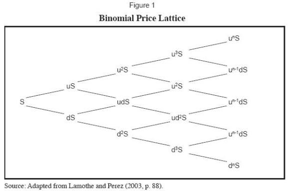
The binomial model as proposed by Cox-Ross-Rubinstein (1979) is preferable to that of Black-Scholes when valuing callable bonds. The main reason for this is that even though closed-form option pricing models (i.e. Black and Scholes) are easier to handle, those models do not capture many of the features required in the valuation of a callable bond. Specifically, the Black-Scholes model is extremely inaccurate in capturing the variations of interest rates throughout the life of the option as well as the embedded value of multiple call options after the first settlement date. Although in practice, when a Binomial Model is taken to the “limit” its results tend to converge with those obtained by Black and Scholes, this occurs because the Binomial Model is simply a discrete approximation of the underlying stochastic differential equation used in Black and Scholes. Given that the Binomial Model distinctive feature is the use of discrete periods, this feature is what gives the Binomial Model a certain advantage over Black and Scholes in the specific case of valuing multiple embedded options in callable bonds. This is so because the model assumes (in the specific case of bonds) that the yield of the security evolves on step to step basis as times passes (Wong, 1993). The Binomial Pricing Model assumes that the underlying asset price or yield evolves in a multiplicative binomial pattern in the following manner:

Any node for the price of the asset (S) in the lattice tree should go up by an upward factor (u) with a probability (P) or by a downward factor (d) with a probability (1-P) for multiple periods in the following manner (Figure 1).

In a similar manner we value the price of the call option using a risk-neutral probability approach at each node of the lattice using the following formula¹:

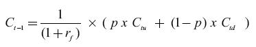
In which C_t-1= Call value for the preceding period

r_f= The proxty variable for the theoretical risk-free interest rate for a given period

C_tu= The call value for the immediately posterior upward node

C_td= The call value for the immediately posterior downward node

P=((1+r_f)-d)/(u-d) or the risk-neutral probability of an upward movement of a replicating portfolio (short or long in a call option, or long or short in risk-free bond) where (u)is an upward factor and (d) is a downward factor.

In order to find the European option value at each node, the formula is applied backwards in each node of the following lattice (based on the nominal value obtained for the option of each node at its maturity) (Figure 2).

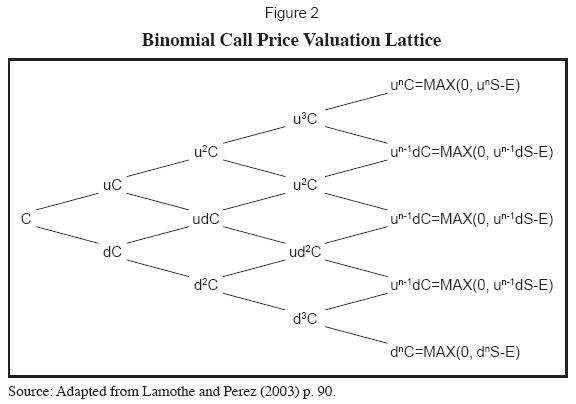
Where E is the strike price of the option being valued at a specific point in time (t), if any value of S is greater than E at maturity the option will be exercised, otherwise its value will be cero (0).

Therefore this approach can be used in valuing multiple embedded options, because by using a lattice we can incorporate irregular and path dependant values during the time to expiration of the option. If indeed, the option is not exercised at a specific node, this means that those cash flows will remain until the next option in the theoretical call schedule expires. By doing this in a repetitive manner, all the calls scheduled in the callable bond will be incorporated into the valuation model. In this way is possible to determine the value of each call embedded on the bond, and how the values of these calls affect the price of the bond and its expected future yield at a specific point in time.

2. A simple methodological approach for implementing the binomial option pricing model for valuing callable bonds: the TGI example²

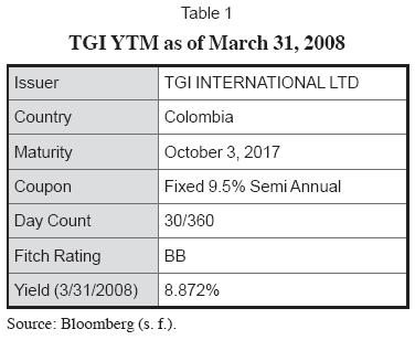
The main problem faced in option valuation is how to find the appropriate proxy variables to be used as inputs of the model. Therefore, the main objective of this paper is to use a practical example on the steps required to value a callable bond using the binomial pricing model. In order to develop a meaningful example of how to develop the binomial pricing model, the example will be focused on the valuation of a recent issue by TGI International Ltd. which is a subsidiary of a Colombian company called Transportadora de Gas del Interior, a local monopoly whose business is the transportation and wholesale distribution of natural gas. The issue has the characteristics presents in Table 1 (Note: For the purpose of this example, and for the remainder of the document, the valuation date is March 31, 2008).

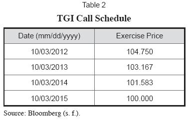
The issue has four embedded call options from the issuer and its call schedule is as follows in Table 2 (it is important to remember that on any coupon payment date the clean price is equal to the dirty price).

The following are some of the problems of how to obtain meaningful proxy variables in order to value this specific issue:

1. Finding a proxy for the risk-free rate, given the fact that even though the issue is dollar- denominated, the company in question is not US based.

2. Finding a proxy for the volatility of the yield of the proxy used as a risk-free rate that incorporates the additional spread required for country risk.

3. Finding a proxy for a non-callable bond issue with the same coupon and maturity date comparable to the issue that is being valued.

4. Finding the spread attributable to specific industry risk.

Therefore, in order to provide a meaningful insight on how to address these issues, a detailed step-by-step methodological approach is described in the process required to value TGI callable bond issue throughout this paper.

2.1 Step 1-Colombian sovereign bonds yield as a proxy variable that incorporates the additional spread required by country risk

Before implementing the lattice approach for predicting the behavior of future yields for the specific case of TGI, it was necessary to find a proxy for a non-callable bond with the same coupon and maturity dates of TGI. Since TGI is located in an emerging market there are no comparable issues from a non-callable bond in order to determine the OAS of TGI. Therefore, in order to find a meaningful proxy for a non-callable bond a synthetic theoretical non-callable bond series was created in order to find a meaningful yield that incorporated both the risk-free rate and a spread attributable to country risk³. This theoretical yield was found through linear interpolation using two Colombian sovereign issues with a maturity date before and after TGI maturity date. The issues have the characteristics presents in tables 3 and 4.

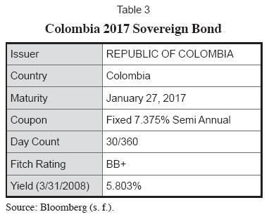
Therefore, the time left to maturity for the Sovereign Bonds expressed in years⁴ is 8.82222 and 11.90 respectively, also the time left to maturity for expressed in years for TGI is 9.50555. Since we know the yield to maturity and the time left to maturity of both bonds, we can use a simple interpolation formula to find the theoretical yield of a Colombian sovereign bond that pays a 9.5% fixed semiannual coupon and matures on October 3, 2017 in the following way:

5.867% = 5.803% + [(9.508333 – 8.82222) × (6.091% – 5.803%)/(11.90 – 8.2222)]

In this way, we find that the theoretical yield for a Colombian sovereign bond with the same maturity date as TGI would be approximately 5.867%. Given that this simple approach has tremendous conceptual flaws we opted to use a more robust term structure model which for this specific case was the Nelson and Siegel model. The Nelson Siegel Model formulation gives a conservative representation of the forward rate function given by (Abad and Benito 2005):

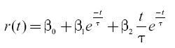
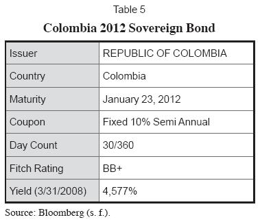
Where the parameters β₀, β₁, β_2, and τ are obtained by finding the rate for a time (t) for different maturities and by maximum likelihood fitting the rate obtained by the formula to the actual observation by minimizing the MSE for each actual vs. calculated observation for the term structure for an observable time period for which our specific case was one year. For calculating the term structure we used the issues presents in tables 5, 6, 7, 8 y 9.

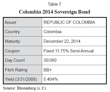
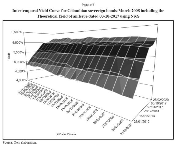
Once the optimal parameters in the Nelson Siegel were found for the date 3/31/2008 by making (t) equal to the time left to maturity of TGI (9.50555 years) we found that the theoretical yield for a Colombian sovereign bond with the same maturity date as TGI using Nelson and Siegel was approximately 5.867%, the difference between the rate found using Nelson and Siegel and that found by using a simpler linear interpolation was just 0.0002%. In average, for the observed period of one year, the difference between the results obtained by simple linear interpolation and Nelson and Siegel was just 0.0187%. The behavior of the intertemporal term structure of the Colombian sovereign bonds can be observed in Figure 3.

2.2 Step 2-Theoretical Colombian sovereign bond yields as a proxy variable for volatility estimates

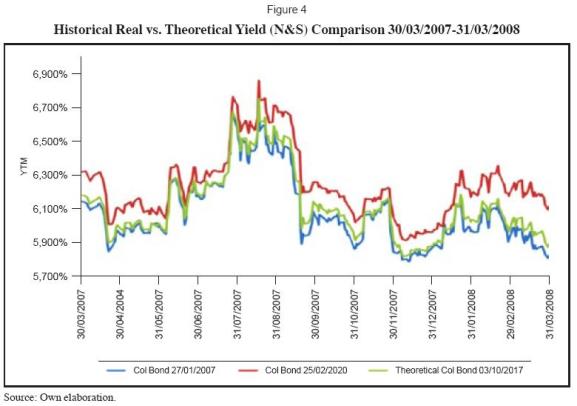
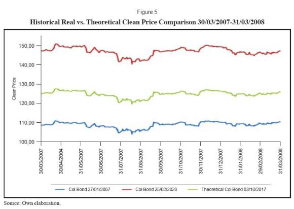
Once we found the approximate theoretical yield of a non-callable Colombian sovereign bond, we can use the same process for creating a synthetic historical series in order to measure the behavior of the volatility of that theoretical bond in the past. The dataset⁵ for obtaining the theoretical yields was formed by the historical closing prices and yield observations of the 2017 and 2020 Colombian sovereign issues from March 30, 2007 until March 30, 2008. Nelson and Siegel was used to obtain a theoretical yield was found for each observation that comprised the dataset. Once the yield was obtained, we found the clean price of the theoretical bond for each date. The summary of the historical price and yield behavior for the two sovereign bonds as well as the theoretical bond are compared in figures 4 and 5.

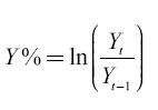
Since the yield is the determinant of price in a bond, we proceeded to calculate the volatility of the yield of the theoretical bond in the following way, on the assumption that the yields are continuously compounded:

Daily yield variation is found using the following formula:

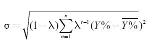
Once we have found the daily yield variations, we can calculate the daily volatility

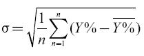
Where n is the number of observations in the dataset and Y% is the average daily volatility.

For our specific example our daily volatility is equal to 0.702539% since the effective trading days for the bonds were 262 and assuming constant volatility we can turn our daily volatility into annual volatility in the following way:

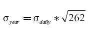
Therefore our annual standard deviation is 11.372%, and we can obtain the semiannual volatility in the following way:

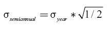
The semiannual volatility for our theoretical sovereign bond would be 8.04093%, also because we know that there are 3 days for the next semiannual coupon in the TGI case using the same formula we find that the expected volatility for the next three days is equal to 1.21683%. Given the fact that sovereign bonds of emerging markets do not trade frequently, reliance on historical prices alone can lead to over-or under-estimation of the volatility of the bond. In order to correct this distortion so we can obtain a better esti-mate of the theoretical sovereign bond real volatility, we used the EWMA (Exponentially Weighted Moving Average) model for our volatility estimation (Riskmetrics, 1996) the formula is:

In order to estimate the optimal decay factor (λ) we minimized the RMSE resultant of an initial decay factor of 0.90, and the optimal decay factor (λ) for the period under observation was 0.9982. Unlike yield, where the difference between a simple linear interpolation and Nelson and Siegel was practically insignificant, in the case of volatility the differences between the two methods are significant. By using EWMA the forecast for annual volatility on 3/31/2008 was 7.1342959%, on a semiannual basis it was 5.0447090% and the expected volatility for the next three days was 0.763416%. Given the fact that most of the research on volatility tends to point out that "historic volatility" is the worst predictor of future volatility (Alexander, 2001), we choose the EWMA as the model for the volatility estimates in the present study. Another reason is the fact that since the EWMA model takes gives more weight to the latest observations and to some extent it helps to correct the problems concerning the liquidity of the Colombian sovereign bond market.

2.3 Step 3-Constructing a lattice using the theoretical Colombian sovereign bond yield data and observed volatility

If, for purposes of simplicity, we assume that the yields follow a log-normal distribution (because like prices, yields can never be below zero), then the upward factor required to construct the lattice would be the geometric standard deviation⁶ of the synthetic series or exp(σ); and likewise the downward factor will be the inverse mean or (1/ exp(σ)). Of course this approach for determining the factors assumes that there is no significant variation on the median yield over the life of the option (an assumption that is often violated in practice). Also, a more practical approach would be to use a subjective upward and downward factor based on our feelings about the behavior of the market for the period under study (Wong, 1993). It is important to remember that the yield and the volatility used in this example were those estimated by using Nelson and Siegel and the EWMA as proposed by Riskmetrics.

Therefore, by applying the formula for the geometric standard deviation in our previous results, we can find the expected semiannual and three days volatility for theoretical issue, and the results are in Table 10.

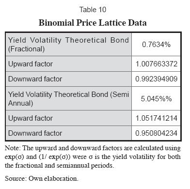
Using the upward and downward factors we can construct the lattice starting from our semiannual theoretical yield of (5.867%/2) = 2.934%. Since the date of the valuation is March 31, 2008 and the next coupon date is April 3, 2008 the upward and downward expected yields for that specific date in the lattice would be 2.934% × 1.007663372 = 2.956% and 2.934% × 0.992394909 = 2.93352%⁷ respectively. For the dates of October 3, 2008 onwards we use the semiannual factors using our previous yields in the lattice. Therefore for that specific date the yields are 2.956% × 1.051741214 = 3.1089% and 2.93352% × 1.051741214 = 2.8106% for the upward branches, for the downward branches the results are 2.956% × 0.950804234 = 2.8106% and 2.93352% × 0.950804234 = 2.7892%. The summary of the results are shown in table 11.

2.4 Step 4-Finding a theoretical discounted non-callable sovereign bond price lattice using the future expected yield behavior lattice

The first step in finding the discounted noncallable sovereign bond price is to calculate the risk-neutral probabilities for a replicating portfolio at each node. The upward and downward risk neutral probabilities are found using the semiannual and three days observed theoretical rate of 2.934% and 0.049% = (2,934% × 3/180) as follows:

Upward risk-neutral semiannual probability = (1 + 2 2.934% - 0.950804234)/1.051741214 - 0.950804234) = 77.802%

Downward risk-neutral semiannual probability = 1 - 77.802% = 22,198%

The same procedure is applied to the three days rate and factors:

Downward risk-neutral semiannual probability = 1 - 53.011% = 46.989%

The theoretical price of the bonds is found discounting the principal and the coupons independently in a backward manner. As we can observe form the yield lattice on April 3, 2017 we have a total of 210 possible branches (or expected yields). For the date of October 3, 2008 or the date of expiration of the bond we can expect to receive a notional principal of 100 for the 21 possible branches on that specific date, in the same way as the principal, we can expect to receive a coupon of 4.75. As observed from the yield lattice in April 3, 2017 the highest yields expected in the upward branches are 7.329% and 6.626% respectively. Therefore, the expected principal price for those yields in April 3, 2017 are 100/(1 + 7.329%) = 93.17116911 and 100/ (1 + 6.626%) = 93.78581492. In this way we can find the expected price for the upward branch on October 3, 2016 by discounting the expected prices for April 3, 2017 and applying the risk-neutral semiannual probability for each price in the following way:

Expected price on October 3, 2016 = (77.802% × (93.17116911/(1 + 6.969%⁸)) + (22.198% × (93.78581492/(1+6.300%)) = 87.35128424

For the coupons the procedure is the same as that used for the principal with the difference that we accrue the coupons of each period. From the yield lattice, we can observe that in April 3, 2017 the highest yields expected in the upward branches are 7,329% and 6,626% respectively. Therefore, the expected accrued coupon prices for those yields on April 3, 2017 are (4.75/(1 + 7.329%)) + 4.75 = 9.175630533 and (4.75/(1+6.626%)) + 4.75 = 9.204826209. In this way we can find the expected accrued coupon prices for the upward branch on October 3, 2016 by discounting the expected accrued coupon prices forApril 3, 2017 and applying the risk-neutral semiannual probability for each price in the following way:

Expected accrued coupon price on October 3, 2016 = (77.802% × (9.175630533/(1 + 6.969%) + 4.75)) + (22.198% × (9.204826209/(1 + 6.300% + 4.75))=13.3459363

In this way, we continue to value the principal backwards to April 3, 2008 for valuing the principal and the coupons on the date of March 31, 2008, we use the risk three-day neutral probability and the fractional discount factor for the period (3/180 = 0.01666667) as follows:

Expected price on March 31, 2008 = (53.011% × (49.32627606/(1 + 2.934%) ^0.01666667)) + (46.989% × (52.9608102/ (1 + 2.934%)^0.01666667))= 51.02149867

Expected accrued coupon price on March 31, 2008 = ((53.011% × ((70.26506064/(1 + 2.934%)^0.01666667)) + 4.75))+((46.989% × ((72.45660412/(1+ 2.934%^0.01666667)) + 4.75))= 76.02689315

The expected non-callable price for the theoretical bond would be the sum of the expected price for the principal and coupons on March 31, 2008 that means that the expected non-callable price would be 51.02149867 + 76.02689315 = 127.0483918. In the same way, a theoretical price can be found for each node of the non-callable bond price lattice. In tables 12, 13, and 14 we can observe a summary of the results for the principal, coupons and expected bond prices.

2.5 Step 5-Finding a theoretical call price for each option embedded in the callable bond using the theoretical non-callable sovereign bond price lattice

Once we have the expected non-callable price for each node until maturity we can proceed to calculate the theoretical value for each option embedded on the bond according to the following call schedule (Table 15).

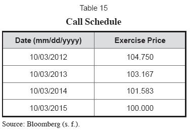
Since the call is priced backwards we begin with the first option that has an exercise price of 104.75 on October 3, 2012. As we can appreciate from the non-callable bond price lattice from the possible 11 expected prices on October 3, 2012, just 8 of them will be in the money, or have an exercise price that is greater than the expected price. Therefore, the possible notional call prices on that date would be as follow: If the exercise price is 104.75 and the expected price on the upward node is 101.6975182, then the call price would be cero because C=MAX(0, 101.6975182-104.75). In the case of the second node, the call price would be 0.7377962 because C=MAX(0, 105.4877962-104.75) and so forth until the call price for each node for an expected noncallable price is found. Then the call option is priced backwards using the semiannual risk-neutral probability in the following way:

Expected Call Price second Node on April 3, 2012 = ((77.802% × 0) + (22.198% × 0.7377962))/(1+4.426%⁹)=0.156835111

Then we continue to price the call backwards to April 3, 2008. For valuing the call option on March 31, 2008, we use the risk three day neutral probability and the fractionate discount factor for the period (3/180=0.01666667) as follows:

Expected Call Price on March 31, 2008 = ((53.011% × 5.35010251)+ (46.989% × 9.06234989))/(1+2.934%¹⁰)^0.01666667))= 4.521392559

It is important to note that in the nodes where the option is exercised, for the next option only the nodes that were not exercised in the first option will be taken into account when valuing the second option scheduled on October 3, 2013. Therefore, the expected prices used to price the second option would be (note that the paths after the exercise of the first option cease to exist because the bond has been recalled by the issuer through the exercise of the first call option) (Table 16).

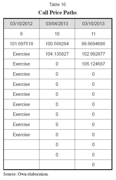
If the second option exercise price on October 3, 2013 is 103.167 and we just have two expected prices for that date, then the notional call prices for the second option would be:

If the stated price for that date is greater than the exercise price of the option of 103.167, the option will be exercised: otherwise the option will be allowed to expire and its value would be zero. With these notional call values, we use the same procedure of the first option to find the value of the second option on March 31, 2008. The third and fourth option call values are found in the same way as the second option (taking into account only the stated prices that have not been exercised in the previous option until the last option expires). The results for the four options are shown in tables 17, 18, 19 and 20:

Therefore, by adding the four option call prices we found that the embedded options of the bond have a total value of 4.521392559+ 0.496152948+0.487039616+0.122441017 = 5.62702614.

2.6 Step 6-Finding the theoretical option adjusted spread for a theoretical Colombian sovereign non-callable bond

Since we know that the theoretical dirty price of a Colombian sovereign bond with a coupon of 9.5% on March 31, 2008 is 127.0483918. Also, we know that the value of the call option in the hands of the issuer is 5.62702614. Therefore, the expected dirty price on March 31, 2008 of a theoretical callable Colombian sovereign bond with the same maturity, coupon and call schedule as TGI would be 127.0483918 – 5.62702614 = 121.4213657. If the bond pays a 4.75% semiannual coupon on April 3, 2008 on a 30/360 basis then the accrued interest up to that date would be ((4.5%/180)×177) = 4.67083333. Therefore, the clean price of our theoretical callable bond would be 122.768876-4.67083333=116.7505323 and the expected yield of a theoretical Colombian sovereign callable bond would be as Table 21.

If we know that the spread of a Theoretical non-callable Colombian Sovereign Bond on March 31, 2008 is 5.867% then 7.052% – 5.867%= 1.185% or approximately 118.85 basic points are attributable to the value of the call options that the investor in theory “sells” to the issuer which is the value of the OAS in this specific example. Similarly, if we know that on March 31, 2008 the market yield of TGI is 8.872%, and we already know the theoretical OAS for a Theoretical Colombian sovereign bond, then we can assume that the difference in spread can be attributable to the company-specific risk of a natural gas company operating in Colombia. In this case this risk can be valued as an additional spread of 8.872%–7.052%=1.820% or approximately 182 basics points. For investment strategy purposes, if we can assume that the company specific risk is constant and that changes in yield are attributable to the country risk and the OAS of the bond on a following date, then we can verify if the callable bond is overpriced or underpriced on that date depending on the expected theoretical OAS or country risk variation.

Conclusions

This paper presents a complete detailed methodological approach for valuing callable bonds in Emerging Markets. Through the development of a practical example using the binomial pricing model, it was possible to determine what the theoretical value of the Option Adjusted Spread of TGI would be. Moreover, by using meaningful proxy variables taken from real-life data, it is possible to find better estimates of the spread attributable to specific risk of companies operating in emerging markets. Although, it is important to remember that in periods of high volatility or market unrest in which the value of the option increases or decreases in an abrupt manner, it would be possible to obtain a negative country risk premium. However, the question remains, whether in a time of market turbulence this premium changes in a manner which is positively correlated with the Colombian sovereign bond discount rate. Also, and of special importance, there is the determination of a theoretical sovereign price for a bond that has the same country of origin as the company whose callable bond issue we wish to value. Another important question for future research is to compare the consistency of the results obtained using Nelson and Siegel vs. other term structure models such as Vasicek or its extended version developed by Hull and White. Finally, by applying a commonly-used methodology such as the binomial pricing formula, we expect to prepare the ground for further research on how to develop methodological approaches on how find meaningful proxy variables for complex valuation models using real market data.

Footnotes

1. For a complete development of the algebraic process necessary for finding risk-neutral probabilities and the theoretical background of the principles behind the replicating portfolio inherent in the binomial option pricing formula, we recommend the book Opciones financieras y productos estructurados (2003), by Prosper Lamothe Fernández and Miguel Pérez Somalo, pp. 79-90.

2. Although (Ritchken, 1995) made a well-augmented point over the advantage of trinomial trees over binomial trees on the grounds that with an additional degree of freedom move spacing can be independent over move timing a trinomial tree. This advantage offers a better approximation for short term options. In the long term such differences are negligible and both models tend to converge. For more relevant information on the subject we recommend the working paper "On the Relation Between Binomial and Trinomial Option Pricing Models" written by Mark Rubinstein (2000) and that is available at the following website: http://www.haas.berkeley.edu/groups/finance/WP/rpf292.pdf.

3. In other words, a yield that incorporates the required country risk spread over a US treasury with similar maturity.

4. To obtain the exact time from the 31 of March 2008 until the date of maturity, we first calculate the time left in a semiannual basis (S/A basis), this is done in order to take into account all the coupons left as well as the principal. Then we express the time in an annual basis, because the yields are expressed by the market in an annual basis. Also the fraction is to denote the time left from the current date until the next coupon payment. In the specific case of TGI, in a semiannual basis, this fraction is expressed as 0.0166667. That gives us in total 19.0166667 semiannual periods that divided by two gives us 9.508333 years.

5. Each dataset was comprised of 262 observations.

6. The geometric standard deviation is defined as the exponentiated value of the standard deviation of the log transformed values

7. The results in the lattice are rounded up to three decimal places, so 2.93352% would be presented as 2.934% in the lattice.

8. The yields used to discount this node are those in the upward branches of the yield lattice for October 3, 2016.

9. This is the yield found in the first node on April 3, 2012

10. This is the yield found in the first node on March 31, 2008 in the yield lattice.

References

1. Abad, P. and Sofia B. (2005). Using the Nelson and Siegel model of the term structure in value at risk estimation. Working paper. Barcelona: Universidad de Barcelona.         [ Links ]

2. Alexander, C. (2001). Market models (1^st ed.). West Sussex: John Wiley and Sons.         [ Links ]

3. Bloomberg System, Government and Corporate Modules (s. f.). Consultation date: April 4 2008.         [ Links ]

4. Claude, E; Campbell, H. and Tadas, V. (1992). New perspectives on emerging market bonds. Journal of Portfolio Management, 25 (2), 83-92.         [ Links ]

5. Cox, J.; Ross, S. and Rubinstein, M. (1979). Options pricing: A simplified approach. The Journal of Financial Economics, 7 (September), 229-263.         [ Links ]

6. Dolly, T. (2002). An empirical examination of call option values implicit in U.S. corporate bonds. Journal of Financial and Quantitative Analysis, 37, 693-720.         [ Links ]

7. Edleson, M. E.; Fehr, D. and Mason, S. P. (1993). Are negative put and call option prices implicit in callable treasury bonds? Working paper. Boston: Harvard Business School.         [ Links ]

8. Eichengreen, B. and Ashoka M. (1999). What explains changing spreads on emerging market debt: fundamentals or market sentiment? In S. Edwards (Ed.), Capital inflows to emerging markets. Chicago: University of Chicago press.         [ Links ]

9. Henderson, T. M. (2003). Fixed income strategy (1^st ed.). West Sussex: John Wiley and Sons.         [ Links ]

10. Lamothe P. and Pérez Somalo, M. (2003). Opciones financieras y productos estructurados (2^nd ed). Madrid: McGraw Hill.         [ Links ]

11. Longstaff, F. A. (1992). Are negative option prices possible?: The callable U. S. treasury bond puzzle. Journal of Business, 65, 571-592.         [ Links ]

12. Ritchken, P. (1995). On pricing barrier option. Journal of Derivatives, 3 (2), 19-28.         [ Links ]

13. Rubio, F. (2005). Valuation of callable bonds: The Salomon Brothers Approach. Recovered on July 2005, of http://ssrn.com/abstract=897343.         [ Links ]

14. Wong, A. M. (1993) Fixed income arbitrage: Analytical techniques and strategies (1^st ed.). West Sussex: John Wiley and Sons.         [ Links ]