^* This article is the product of scientific research that started on 24 June 2010 and ended on 11 September 2010. The executing and financing institution is Universidad Tecnológica de Bolívar, Instituto de Estudios para el Desarrollo (IDE). The article was received on 28-09-2010 and was approved on 27-10-2010.

^** MSc. in Industrial Engineering, University of Missouri, Columbia, Missouri, USA, 1969; BSc in Industrial Engineering, Universidad de los Andes, Bogotá, Colombia, 1967. Associate professor in the Faculty of Economic and Administrative Sciences, Instituto de Estudios para el Desarrollo (IDE), Universidad Tecnológica de Bolívar, Cartagena, Colombia. e-mails: nachovelez@gmail.com, ivelez@unitecnologica.edu.co.

ABSTRACT

This article (1) identifies three sources of risk for tax shields (TS): Two of them are associated with debt risk and one is associated with operating risk. (2) Aset of conditions for defining risky debt associated with cash flow, not with earnings, is presented. (3) It further shows that realization of TS for finite cash flows in a period of time t is correlated with Earnings before Interest and Taxes (EBIT) plus Other Income (EBITO), not with interest expenses at time t. With the results of a Montecarlo Simulation the behavior of TS, Cash Flow to Debt and EBITO are examined. In conclusion, the article suggests that it is not reasonable to define the risk of TS as measured by a single discount rate, but rather as a mix of debt risk and operating risk.

Key words: Weighted average cost of capital, firm valuation, tax shields, cash flows, Montecarlo Simulation, discount rate for tax shields.

RESUMEN

Este documento identifica tres fuentes de riesgo para el escudo fiscal o ahorro fiscal (AI): dos de ellos están asociados con el riesgo de la deuda y un riesgo operativo, relacianado con la operación de la firma. Se presentan, además, unas condiciones para definir la deuda con riesgo asociado al flujo de efectivo y no a las ganancias contables. La realización efectiva de los escudos fiscales para flujos de caja finitos en cualquier período t se correlaciona con la utilidad operativa (UO) más otros ingresos (EBITO) y no con los gastos de interés en t. Con los resultados de una simulación de Montecarlo se examina el comportamiento de los escudos fiscales, del flujo de caja de la deuda y la EBITO. En conclusión, no es razonable definir el riesgo del AI, medido por una sola tasa de descuento, sino como una mezcla de riesgo de la deuda y el riesgo operacional.

Palabras clave: Costo promedio ponderado del capital, valoración de la empresa, amparos fiscales, flujos de caja, simulación de Montecarlo, tasa de descuento para amparos fiscales.

RESUMO

Este estudo (1) identifica três fontes de risco no que diz respeito aos incentivos fiscais: dois deles estão associados com o risco da alavancagem e um associado de risco operacional; (2) são apresentadas umas condições para a definição do risco de alavancagem, associadas ao fluxo de caixa e não ao lucro contábil é apresentado, e (3) mostra que a realização de incentivos fiscais para os fluxos de caixa finito em qualquer período de tempo t são correlacionados com lucro antes dos juros e impostos, além de outras receitas (EBITO), mas não com as despesas de juros no tempo t. Com os resultados de uma simulação de Montecarlo é estudado o comportamento dos incentivos fiscais, do fluxo de caixa da dívida e do EBITO. Como conclusão, não é razoável definir o risco dos incentivos fiscais através de uma única taxa de desconto, mas como uma mistura de risco de alavancagem e risco operacional.

Palavras chave: Custo médio ponderado do capital, valorização da empresa, incentivos fiscais, fluxo de caixa, simulação de Monte Carlo, taxa de desconto para incentivos fiscais.

Introduction

In current financial literature the volatility of tax shields (TS) from debt is usually associated with debt risk. This paper suggests that the volatility of tax shields is also associated with operating risk. The existence of Earnings before Interest and Taxes (EBIT) plus Other Income (OI) (EBITO, for short) is what makes it possible for the firm to earn tax shields. Interest expenses are the origin of debt tax shields; however, the realization of TS depends on EBITO. This is relevant because TS plays a crucial role when defining cash flows and cost of capital for valuation purposes.

This work is organized as follows: Section One reviews relevant literature. Section Two studies Cash Flow to Debt (CFD) and in particular the interest expenses and tax shields (TS). In this Section sources of TS risk are identified and a critique to the Miles and Ezzell (1985)'s proposal is presented. Section Three, with the results of a Monte Carlo Simulation (MCS), examines the behavior and relationships of tax shields, CFD and EBITO. Section Four summarizes the findings. There are four appendixes that explain the financial planning model used, the descriptive statistics resulting from the MCS, the derivation of conditions for default and the derivation of an algorithm to calculate TS.

1. Literature review

There are several approaches to discounting tax shields. One of them establishes that tax shields should be discounted at the cost of debt (more precisely at the risk free cost of debt), see for example, Modigliani and Miller (1958, 1963), Myers (1974), Luehrman (1997), Brealey and Myers (2003), and Damodaran (2002, 2005). Another school of thought says that the discount rate for tax shields should be the unlevered cost of equity, see for instance, Harris and Pringle (1985), Ruback (2002), Tham and Vélez-Pareja (2001, 2004). Finally, Miles and Ezzell (1985) and Arzac and Glosten (2005), propose to discount tax shields at the cost of debt for year t and at the cost of unlevered equity for all subsequent years from t+1.

Regarding the behavior of tax savings, Cordes and Sheffrin, (1983), Dammon and Senbet (1988), Graham (2000), and Grabowski (2009) report that some firms do not fully use their tax shields in the current period but receive them in the future when losses carried forward are permitted.

Newbould, Chatfield, and Anderson (1992) and Kaplan and Ruback (1995), Fama and French (1998), Graham (2000), and Kemsley and Nissim (2002) agree that tax shields are relevant and might account for a good part of a firm´s value.

2. Understanding cash flow to debt and tax shields

This section examines cash flow to debt, tax shields and the sources of risk for tax shields; it also contains a digression on the Miles and Ezzel (1985) proposal.

2.1 Cash flow to debt

Cash flow to debt (CFD) is what debt holders lend to the firm and/or receive back from the firm when loans are repaid. The CFD has two components: (1) interest payments and (2) met principal payments/loans inflows. Interest payments in t are calculated on the amount of debt D_t-1. This means that interest charges are fully known at t–1, assuming constant cost of debt. Interest payments are:

I_t = KdD_t-1 (1)

Where I is interest charge, Kd is the cost of debt and D is debt.

Alternatively, net principal payments/loans inflows are an item defined in time t. In case of deficit, a financial planning model will define when and how much debt should be acquired and when to pay the principal. In other words, this portion of CFD is based on situations that occur and/or decisions made at time t. Deficits depend on sales revenues, expenses, capital investments and the like. That is, they depend on the operating and investment activities of the firm.

2.2 Proper calculation of tax shields

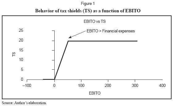
Wrightsman (1978) and Vélez-Pareja (2009 and 2010) propose an algorithm for calculating tax shields. It is of interest to analysts when forecasting financial statements and cash flows to estimate values of firm and equity. While interest charges are fully known at any t-1 assuming constant cost of debt, tax shields are not. Tax shields at t depend on EBITO and are a piecewise-defined function of it, as follows:

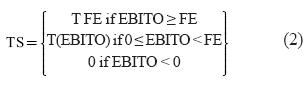
TS is tax shields, FE is financial expense, T is corporate tax rate and EBITO is EBIT+OI. This piece wise-defined function is depicted in Figure 1. See derivation in Appendix D.

The right to earn tax shields occurs when interest is subtracted and deduced in the Income Statement, not when interest is paid. In other words, a firm could never pay the accrued interest and still retain the right to the tax shield. However, the firm actually receives the tax shields when taxes are paid. Tax shields reduce the amount of taxes paid, compared to the situation of an unlevered firm. For a better understanding of these ideas, Table 1 shows the conditions for interest, tax shields and taxes for actually earning the TS.

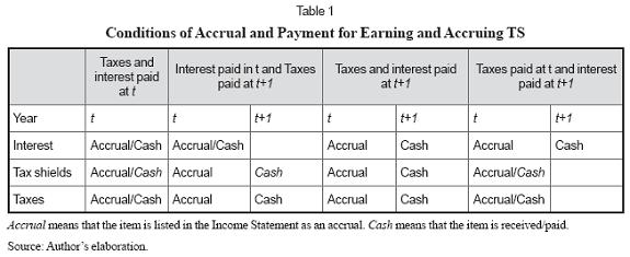
The above table indicates when each item is accrued and/or is paid/received. Observe that in all cases the right to earn tax shields occurs when interest and taxes are accrued, no matter whether interest is paid or not. Note also that TS are received only when taxes are paid.

Another way to understand the idea of the right to earn tax shields when interest/taxes are accrued is to think of what happens when losses carried forward (LCF) are permitted. The firm that has financial expense (interest charges) has the right to earn the tax shields (T times financial expense) but when EBITO is zero or negative (the extreme case) the tax shields are apparently lost because taxes are zero. However, when LCF are permitted, the tax shields corresponding to the year when EBITO was negative can be recovered when losses from previous years are carried forward to a future year where the firm has enough Earnings before Taxes (EBT) to offset previous losses.

2.3 Sources of tax shields risk

Wrightsman defines risky debt "in terms of the possibility that EBIT may turn out not to fully cover interest expense. If some possible EBIT outcomes from a given probability distribution of EBIT fall short of interest, then interest can fall into jeopardy, and debt is risky" (1978, p. 652).

On the other hand, Talmor, Haugen and Barnea (1985) consider the conditions for risky debt are associated with cash flow, not with EBIT. They suggest, however, that the tax deduction and tax shields are obtained when the firm pays the interest charges and not when the firm accrues the financial expense and pays taxes. Generally Accepted Accounting Principles (GAAP) require companies construct their financial statements according to the accrual method, and hence, the tax deduction (and the tax shields) is obtained on an accrual and not on a cash basis.

Tax shields have two sources of risk: debt risk and operational or realization risk. Debt risk is associated with cash flows (from Cash Budget or Cash Flow Statement) and operational risk is associated with EBITO, from the Income Statement.

Debt risk has two components: Market or systematic risk and default risk. Creditors estimate the level of default risk (probably looking at leverage and other items) and add it to the risk free rate to obtain the cost of debt. Market or systematic risk is associated to the volatility of Kd, the cost of debt. Insolvency occurs if there is not cash availability and this is measured with the Cash Budget or Cash Flow Statement, not with the Income Statement. In fact, the firm will pay interest either from operating income or from other sources in order to avoid insolvency. Interest can be paid out from internally generated funds such as depreciation, from other debt or from new equity investment.

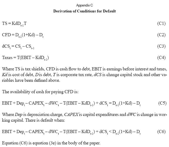
Assuming that losses carried forward are not permitted, and given the residual characteristic of cash flow to equity (CFE), the firm will default when the following general conditions are fulfilled, from the point of view of cash flow:

EBIT + Dep_t - CAPEX_t - dWC_t - T(EBIT - KdD_t-1) + dCS_t < D_t-1(1+Kd) -D_t (3a)

Where Dep is depreciation charges, CAPEX is capital expenditures, dWC is change in working capital, dCS is the change in capital stock and other variables have been defined above (see Appendix C). However, the firm will default under four scenarios:

Case 1. EBIT ≤ Interest charges and CAPEX zero:

EBIT + Dep_t - dWC_t + dCS_t < D_t-1(1+Kd) - D_t (3b)

Case 2. EBIT > Interest charges and CAPEX zero:

EBIT(1-T) + Dep_t - dWC_t + TKdD_t-1 + dCS_t < D_t-1(1+Kd) - D_t (3c)

If CAPEX ≥ Dep there are two additional cases:

Case 3. EBIT ≤ Interest charges:

EBIT - (CAPEX - Dep) - dWC_t + dCS_t < D_t-1(1+Kd) - D_t (3d)

Case 4. EBIT > Interest charges:

EBIT(1-T) - (CAPEX - Dep) - dWC_t + TKdD_t-1 + dCS_t < D_t-1(1+Kd) - D_t (3e)

The derivation of (3e) is presented in Appendix C.

This idea complements the proposal from Talmor, Haugen and Barnea (1985). From these conditions for default it can be seen that the criteria for defining risky debt com-paring EBIT and financial expense are not appropriate. Insolvency does not occur because EBIT or EBITO falls short of interest.

The other source of tax shields risk is when EBITO outcomes from a given probability distribution are lower than interest. This is exactly what equation (2) is showing. Even with a risk-free debt, tax shields might be risky due to EBITO. A firm might have a risk free debt (from the standpoint of cash availability) and yet, tax shields are risky (from the Income Statement point of view). Put differently, EBITO could be greater than financial expense and yet, the firm could default and hence, debt is risky. EBITO is calculated on an accrual basis. Insolvency is related to cash flow and to cash availability.

The fact that D is known at t-1 and that interest is fully known at that time assuming constant cost of debt, does not mean that tax shields are certain or riskless, nor that debt is riskless. Tax shields depend on EBITO which is a random variable that depends in turn several on other variables such as prices, inflation, increase in units sold, expenses, etc.

In summary, tax shields risk depends on EBITO and this risk is independent of debt risk in the sense explained above: the firm could have a risk free debt and yet have a risky tax shields. Tax shields are associated to the accrual of interest. On the contrary, tax shields are received when taxes are paid, not when interest are accrued or when interest is paid. This said, three sources of risk are identified and associated with TS risk:

• Risk of default in debt¹. There exists a possibility that there is not enough cash to pay interest and/or principal. If the default is such that the firm does not pay the accrued taxes (default in taxes), it will not earn the TS (on a cash flow basis). This means risky debt and risky TS. If the firm defaults in debt and not in taxes, it means risky debt but it might effectively earn TS. Observe that the default risk is not only the situation of insolvency that prevents the firm from paying debt and/ or interest. It might occur when the firm pays the bank but does not pay taxes. If the firm does not pay taxes, it will not earn the tax shields. Tax shields are earned when taxes are paid (see Table 1).

• Market cost of debt risk². Variable Kd is subject to systematic risk. The market rate could change and that is a source of risk for the TS. However, what creates TS is not the market rate but the contractual rate. Unless there is a link between the contractual rate and the market rate the risk of Kd (market rate) does not affect Kd contractual. There is one way to link that rate to market rate: to index the contractual rate to inflation. This means risky debt and risky TS. As we are interested on the variability of TS as an element to define its risk, the critical issue is the variability of contractual rate (the rate the firm uses to pay interest).

• Operational³ or realization risk of TS is associated with EBITO and the financial expense. This is a clear dependence of TS from EBITO. This is the piecewise function of TS as a function of EBITO (see eq (2)). This means risky TS. This can be seen in Figure 2.

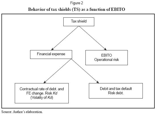
From Figure 2, it can be said:

• A debt is risk free if the installments are certain. If debt is at perpetuity, then the installments are interest payments. A debt is risky if it is not risk free.

• The TS is risky if the stream of TS is not known with certainty. Then

• A risk free debt does not imply a risk free TS.

The proof is evident: if the debt is risk-free, then FE is fixed, so TS is a function of EBITO (see piecewise function, above). But (EBITO) is a risky variable, which implies that TS is risky as well. See equation (2) above.

In other words, a risky market cost of debt implies risky TS, and non-risky debt does not imply risk free TS. And vice versa: risky TS do not imply risky debt. Risk free TS imply EBITO greater than financial expense, risk free cost of debt and risk free debt.

2.4 The M&E proposal

Miles and Ezzel (1985) assume that as D is known in t, interest charges at t are fully defined and hence tax shields at t+1 are risk free and tax shields from t+1 will not be risk free and will be as risky as the FCF afterwards.

As in t-1 it is not known in advance on which interval in (2) EBITO will occur in t, the conclusion is that TS are risky although interest charges are fully known. This risk has to be taken into account when defining the discount rate for TS. Lewellen and Emery (1986) have the same understanding: the risk of tax shields comes from the certainty or uncertainty of the interest charges. Interest charges might be fully known and that does not make tax shields risk free. What makes tax shields risk free given a risk free debt, is the certainty that EBITO is greater than or equal to financial expense. If EBITO is not known in advance (at time t-1) then tax shield are risky and the assumption of Miles and Ezzel has limited application. The next section examines the behavior of tax shields compared with EBITO and with CFD.

3. A Monte Carlo simulation

A selected a sample for non financial firms (for year 2009) from Superintendencia de Sociedades (the Colombian supervisor and regulator for non-traded firms) was examined. Table 2 depicts the sample disaggregated considering EBITO and compared with Other Expenses (OE). Due to lack of disaggregated data, the assumption is that OE are 100% financial expense. Financial expense include interest expenses, bank commissions and exchange losses, and other expenses.

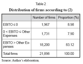
The above table shows that 8.98% of firms lose their debt tax shields, 7.90% earns less than full tax shields, and only 83.12% earn full tax shields. This means that a significant number of them (almost 17%) lose or at least postpone part or all of the benefits of tax shields from debt payment. This is in line with the findings of Cordes and Sheffrin, (1983), Dammon and Senbet (1988), Graham (2000) and Grabowski (2009).

Using equation (2) the third section of TS is calculated as T FE and it is strictly related to debt risk. The proportion of this section with the other two (related to operating risk) is 4.92 (83.12%/16.88%).

We now explore the relationship between EBITO, CFD and TS, the items that are affected by the sources of TS volatility. The purpose of examining this behavior is to shed light upon the risk associated with TS. The exploration uses simulations of CFD, EBITO and TS.

As mentioned in Section One there is a debate on which a discount rate should be used to discount TS. As can be seen in their general formulas, cost of equity and average cost of capital depend on this discount rate. See Taggart (1991) and Tham and Vélez-Pareja, (2004) as follows.

and

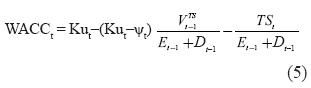
Where Ke is the cost of levered equity, Ku is the cost of unlevered equity, Kd is the cost of debt, D is market value of debt, E is market value of equity, ψ is the discount rate for the tax shields (TS), V^TS is the present value of TS at ψ and WACC is the weighted average cost of capital.

Observe that equations (4) and (5) are quite different from the traditional and widely used textbook formulas for cost of capital. This means that the greater the debt TS lost or postponed, the higher the cost of capital and the greater the risk of overestimating the valuation of cash flows if the appropriate formula for the cost of capital and cash flows are not used.

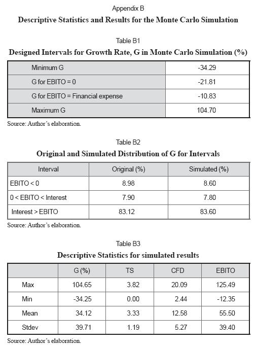
A Monte Carlo Simulation scenario was designed with the results of Table 2. Based upon a hypothetical financial planning model 1,000 simulations were made with growth in units as input variable and TS, CFD and EBITO as output variables. Two critical points were estimated: one point is the growth rate, G, where EBITO is zero and the other is where EBITO matches Other Expenses. These two points were identified using reverse engineering (Goal seek in a spreadsheet). With this information a typical profile in terms of EBITO and Other expenses was constructed in order to examine their behavior. These two critical points define the intervals in the piece-wise equation (2). The intervals are

• Interval 1 is defined from a minimum G to a second level of G associated to EBITO equal to zero (first critical point, above). Referring to Table 2 it is 8.98% of total interval.

• Interval 2 is defined from the growth rate associated to EBITO equal to zero up to the growth associated to EBITO equal to Other expenses (second critical point, above). The size of this interval is the difference between the two critical points above. Referring to Table 2 it is 7.90% of total interval. Ifthe size of this interval and its proportion on the total interval length is known, we can calculate the minimum and maximum G⁴.

• Interval 3 is defined from the growth rate associated to EBITO equal to Other Expenses to a maximum growth rate. Referring to Table 2 it is 83.12% of total interval.

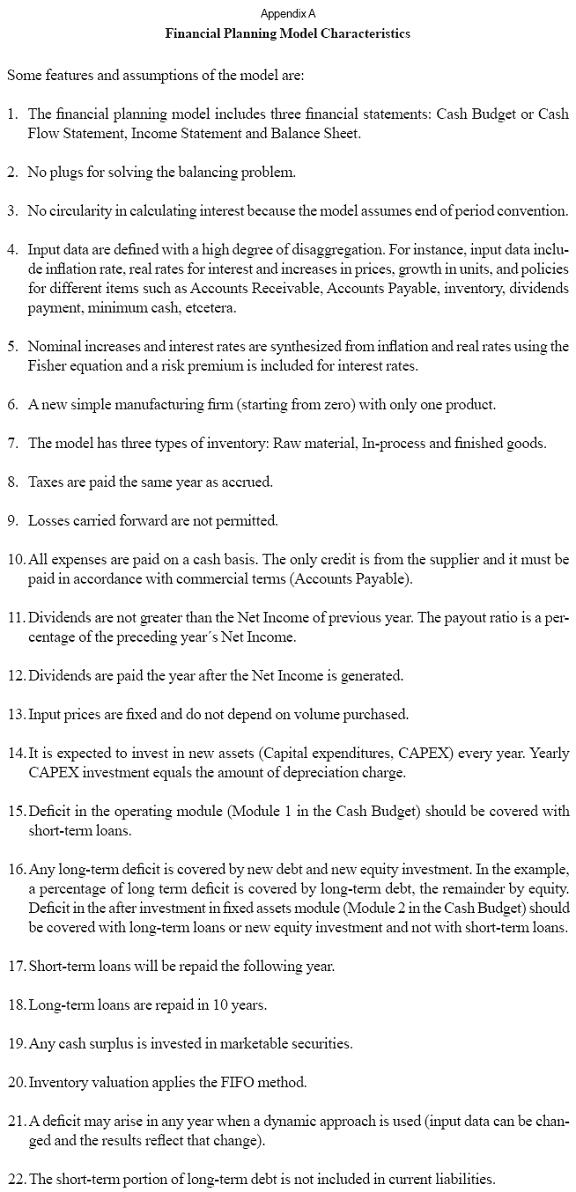
The financial planning model can be downloaded from http://cashflow88.com/decisiones/cige_ME_web.xlsx, The planning model has some characteristics listed in Appendix A.

The probability distribution of the input variable growth in units (G) was assumed as a uniform distribution. Appendix B shows the minimum and maximum values of real growth for running the simulation.

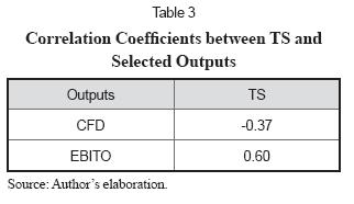
As has been discussed, TS risk has two sources: debt and operating results. For that reason Table 3 shows the correlation coefficients among TS, CFD and EBITO. CFD includes interest payment that is the basis of TS calculation and EBITO includes the operating earnings (EBIT).

If the relationship among TS, CFD and EBITO were linear, then it can be expressed as:

TS = β₀ + β₁CFD + β₂EBITO + ε (6)

Tables 4a and 4b show the Ordinary Least Squares (OLS) regression for eq. (6).

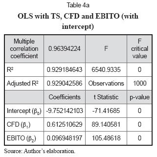
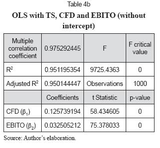
Results from OLS suggest, as expected, from Table 2 and equation (2), that the discount rate for TS is a mixture of debt risk and operating risk. As it has been suggested, the sources of TS risk are debt risk and operational risk. The non intercept model in Table 4b depicts the proper relationship among TS, CFD and EBITO. In this case, the contribution of debt risk to TS is 3.87 (0.125739194/0.032505212) times the contribution of operational risk.

A naïve approximation to the elusive discount rate for TS is to weight the risk of debt (default, for instance) and the risk associated with EBITO (2) as in (7):

ψ = W_drKd + W_EBITOKu (7)

Where ψ is the discount rate of TS, W_dr is the weight for the possibility of debt default and volatility of Kd, W_EBITO is the weight for operating risk (Ku), associated to EBITO. To have an idea of the probability of default to be included in a naïve approach as the previous one, Table 5 shows the proportion of US firms that are under Chapter 11.

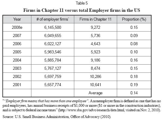
The average of 0.14% could be considered as the probability for a firm to be included in Chapter 11 for defaulting. With this probability one could work out the effect of the risk of debt for default in the naïve approach.

The information regarding the number of firms in Colombia is volatile depending on the inclusion or not of micro enterprises or not. According to information from the World Bank (2010), there are nearly 500,000 formal incorporations in Colombia The latest data is shown in Table 6.

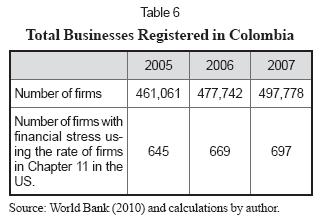
From public information (see Viana Rojas, 2009; El Tiempo, 2004) it is known that from January 2000 to July 2004, there were 964 firms which filed for bankruptcy or arrangement with creditors (210 firms per year). Only in 2000 there were 360 firms that declared financial distress. This means that even 0.14% the rate of firms in Chapter 11 in the US, is an overestimation of what occurs in Colombia in terms of bankruptcy rate. If the average of firms per year (210) is doubled to assess the bankruptcy rate from 2005 to 2007, that rate is 0.09%. Three practical approaches are suggested for estimating W_rd and W_EBITO in eq. (7):

• According to the intervals as shown in Table 2. In this case, W_rd = 83.12% and W_EBITO = 16.88%.

• According to the regression coefficients from Table 4b. In this case W_dr = 79.46% (0.125739194/0.158244406) and W_EBITO = 20.54% (0.032505212/0.158244406).

• According to an estimation of the probability of default. In this case, W_dr = 0.09% and W_EBITO = 99.91%.

Other sophisticated approaches could be considered. For instance, one possible approach is to assume that TS is a contingent cash flow or a real option and working with risk neutral probabilities or considering the TS as a portfolio with different risks and weight and estimate a composite beta and applying the Capital Asset Pricing Model. See Díaz and Vélez-Pareja (2010). All this is beyond the scope of this exploratory work.

In a work in process, Kolari and Vélez-Pareja (2010) have identified a flaw in the traditional Modigliani and Miller's model for valuation. This problem is solved when the discount rate for the TS is Ke, the cost of levered equity. In addition, this approach has the property that Ke captures part of the bankruptcy costs and defines an optimal capital structure. Tham and Vélez-Pareja (2010) developed the formula for Ke when Ke is the discount rate for TS. As seen, there is no clear and specific answer to which is the discount rate for TS.

Concluding remarks

From this work it is possible to draw some conclusions regarding the TS, TS risk, and TS realization as follows:

• Several sources of risk for the tax savings have been identified: risk of debt default, risk of volatility of cost of debt and volatility of EBITO. Conditions for risky debt relate CFD to the available cash and not to earnings (EBIT) that include accruals and in fact do not show the complete cash availability.

• The initial reasoning and critique of Wrightsman, 1978 is supported by the Monte Carlo Simulation results: risk of tax shields includes operating risk and debt risk: operating income (EBITO) and CFD.

• Miles and Ezzell, 1985, proposal is questioned because while the interest charge in t may be known, this does not mean a risk free TS in t+1. Hence, their proposal is limited to very specific scenarios where EBITO is greater than financial expense and when the assumption of EBITO > FE means no risky debt

•There is no clear cut answer to the question about the discount rate for TS.

• There is evidence that in Colombia nearly 17% of firms lost or postponed tax shields in 2009 due to low operational earnings (EBITO). This means that if TS are not defined properly the estimates of their cost of capital estimates might be understated (see (4) and (5)). As a consequence, they are exposed to make sub optimal decisions.

• Available data suggest the rate of bankruptcy filings are much lower in Colombia than in the U.S.

• Using a naïve approach as in (7) and with available data, results are contradictory. Depending on how to assess the weights of debt risk and operational risk, the former could outweigh the latter. This is, TS risk would be closer to debt risk or to operational risk.

• The analysis of the relation among TS, CFD and EBITO should be extended to more years. This paper only explored the behavior as per 2009.

• Other approaches to defining the discount of TS have to be developed. This is not a black and white situation. It might not be possible to assign a single rate of risk to the tax shield as it is subject to different forces that generate risk.

• Finally, Kolari and Vélez-Pareja (2010) report that the risk of TS cannot be less than the cost of levered equity because for discount rates lower than the levered cost of equity, the Modigliani & Miller model presents some flaws for large leverage situations. This eliminates the possibility of using Kd, the cost of debt and Ku, the unlevered cost of equity.

Acknowledgment

I am grateful to Rauf Ibragimov, from Graduate School of Financial Management, Moscow; Carlo Alberto Magni, from University of Modena, Italy, and Gonzalo Díaz, from Universidad Tecnológica de Bolívar, Cartagena, for their comments on this work. The responsibility for the content is entirely mine.

Footnotes

1. The definition of default according to Basel II is "A default is considered to have occurred with regard to a particular obligor when either or both of the two following events have taken place.

• The bank considers that the obligor is unlikely to pay its credit obligations to the banking group in full, without recourse by the bank to actions such as realizing security (if held).

• The obligor is past due more than 90 days on any material credit obligation to the banking group.89 Overdrafts will be considered as being past due once the customer has breached an advised limit or been advised of a limit smaller than current outstandings." (Bank for International Settlements, 2006, p. 100). This criteria does not imply bankruptcy.

2. According to Basel II, "Market risk is defined as the risk of losses in on and off-balance-sheet positions arising from movements in market prices. The risks subject to this requirement are:

• The risks pertaining to interest rate related instruments and equities in the trading book;

• Foreign exchange risk and commodities risk throughout the bank.” (Bank for International Settlements, 2006, p. 157).

In this context we use market risk to refer to the variability of the cost of debt due to effects of the market.

It does not necessarily imply losses. It is related to changes in contractual debt rates.

3. For comparison, Basel II defines Operational Risk as "Operational risk is defined as the risk of loss resulting from inadequate or failed internal processes, people and systems or from external events. This definition includes legal risk, but excludes strategic and reputational risk." (Bank for International Settlements, 2006, pp. 157 and 144). As explained above, operational o realization risk of TS is related to the size and sign not only to the fact that EBITO be negative or positive.

4. (CP₂ - CP₁)/%₂ = TL, CP₁ - G_min = %₁TL, G_max - CP₂ = %₃TL where CP₁ and CP₂ are the critical points found by reverse engineering, %₁, %₂ and %₃ are the proportions of each interval in Table 2. TL is total length of interval.

References

1. Arzac, E.R. and Glosten, L.R. (2005). A Reconsideration of Tax Shield Valuation. European Financial Management, 11 (4), 453-461.         [ Links ]

2. Bank for International Settlements, Basel Committee on Banking Supervision (2006). International Convergence of Capital Measurement and Capital Standards A Revised Framework. Retrieved on November 29, 2010, from www.bis.org/publ/bcbs128.pdf.         [ Links ]

3. Brealey, R.A. and Myers, S.C. (2003). Principles of Corporate Finance (7^th ed.). New York: Mc-Graw-Hill.         [ Links ]

4. Cordes, J.J. and Sheffrin, S.M. (1983). Estimating the Tax Advantage of Corporate Debt. The Journal of Finance, 38 (1), 95-105.

5. Dammon, R.M. and Senbet, L.W. (1988). The Effect of Taxes and Depreciation on Corporate Investment and Financial Leverage. The Journal of Finance, 43 (2), 357-373.         [ Links ]

6. Damodaran, A. (2002). Investment Valuation (2^nd Ed.). Hoboken, N.J.: John Wiley & Sons. Retrieved from: http://pages.stern.nyu.edu/~adamodar/pdfiles/valn2ed/ch15.pdf.         [ Links ]

7. Valuation Approaches and Metrics: A Survey of the Theory and Evidence. (2005). Foundations and Trends in Finance, 1 (8), 693-784. Retrieved from: http://pages.stern.nyu.edu/~adamodar/pdfiles/papers/valuesurvey.pdf.         [ Links ]

8. Díaz, G. and Vélez-Pareja, I. (2010). Estimating the Appropriate Risk Profile for the Tax Savings: A Contingent Claim Approach. Working paper. Retrieved from: http://ssrn.com/abstract=1667621.         [ Links ]

9. El Tiempo (2004, August 10). Ley 55: solo 10 empresas salvadas. Retrieved on Nov 2, 2010, from: http://www.eltiempo.com/archivo/documento/MAM-1591980.         [ Links ]

10. Fama, E.F. and French, K.R. (1998). Taxes, Financing Decisions, and Firm Value. The Journal of Finance, 53 (3), 819-843.         [ Links ]

11. Grabowski, R.J. (2009). Problems with Cost of Capital Estimation in the Current Environment. Journal of Applied Research in Accounting and Finance (JARAF), 4 (1), 31-40.         [ Links ]

12. Graham, J.R. (2000). How big are the tax benefits of debt? The Journal of Finance, 55 (5), 1901-1941         [ Links ]

13. Harris, R.S. and Pringle, J.J. (1985). Risk-Adjusted Discount Rates-Extensions from the Average-Risk Case. Journal of Financial Research (8), 237-244.         [ Links ]

14. Kaplan, S.N. and Ruback, R.S. (1995). The Valuation of Cash Flow Forecasts: An Empirical Analysis. The Journal of Finance, 50 (4), 1059-1093.         [ Links ]

15. Kemsley, D. and Nissim, D. (2002). Valuation of the Debt Tax Shield. The Journal of Finance, 57 (5), 2045-2073.         [ Links ]

16. Kolari, J.W. and Vélez-Pareja, I. (2010). Corporation Income Taxes and the Cost of Capital: A Revision. Working paper. Retrieved from: http://papers.ssrn.com/abstract=1715044.         [ Links ]

17. Lewellen, W.G. and Emery, D.R. (1986). Corporate Debt Management and the Value of the Firm. The Journal of Financial and Quantitative Analysis, 21 (4), 415-426.         [ Links ]

18. Luehrman, T. (1997). Using APV: A Better Tool for Valuating Operations. Harvard Business Review, May-June, 145-154.         [ Links ]

19. Miles, J.A. and Ezzell, J.R. (1985). Reformulating Tax Shield Valuation: A Note. The Journal of Finance, 40 (5), 1485-1492.         [ Links ]

20. Modigliani, F. and Miller, M.H. (1958). The Cost of Capital, Corporation Taxes and the Theory of Investment. The American Economic Review. XLVIII, 261-297.         [ Links ]

21. Corporate Income Taxes and the Cost of Capital: A Correction. (1963). American Economic Review, 53 (3), 443-453.         [ Links ]

22. Myers, S.C. (1974). Interactions of Corporate Financing and Investment Decisions-Implications for Capital Budgeting. The Journal of Finance, 29 (1), 1-25.         [ Links ]

23. Newbould, G.D.; Chatfield, R.E. and Anderson, R.F. (1992). Leveraged Buyouts and Tax Incentives. Financial Management, 21 (1), 50-57.         [ Links ]

24. Ruback, R.S. (2002). Capital Cash Flows: A Simple Approach to Valuing Risky Cash Flows. Financial Management, 31 (2), 85-103.         [ Links ]

25. Superintendencia de Sociedades (2010). Sirem. Retrieved on June 11, 2010, from: http://sirem.supersociedades.gov.co/SIREM/index.jsp.         [ Links ]

26. Taggart, R.A. Jr. (1991). Consistent Valuation and Cost of Capital: Expressions with Corporate and Personal Taxes. Financial Management (Autumn), 8-20.         [ Links ]

27. Talmor, E.; Haugen, R. and Barnea, A. (1985). The Value of the Tax Subsidy on Risky Debt. The Journal of Business, 58 (2), 191-202.         [ Links ]

28. Tham, J. and Vélez-Pareja, I. (2001). The Correct Discount Rate for the Tax Shield: The N-period Case (April). Retrieved from: http://ssrn.com/abstract=267962 or doi:10.2139/ssrn.267962.         [ Links ]

29. Principles of Cash Flow Valuation: An Integrated Market-based Approach. (2004). Boston: Academic Press.         [ Links ]

30. Cost of Capital with Levered Cost of Equity as the Risk of Tax Shields. (2010, August 9). Working paper. Retrieved from: http://ssrn.com/ abstract=1655244.         [ Links ]

31. U.S. Courts (2010). Table F-2: U.S. Bankruptcy Courts. Retrieved on August 7, 2010, from: http://www.rib.uscourts.gov/Docs/Stats/table_f2.pdf.         [ Links ]

32. U.S. Small Business Administration (2010). Statistics of U.S. Businesses, Business Dynamics Statistics, Business Employment Dynamics, and Nonemployer Statistics. Retrieved on Nov. 2, 2010, from: http://www.sba.gov/advo/research/data.html.         [ Links ]

33. U.S. Small Business Administration, Office of Advocacy (2010). Private Firms, Establishments, Employment, Annual Payroll and Receipts by Firm Size, 1988-2007 (table).Retrieved on August 7, 2010, from: http://www.sba.gov/advo/research/us88_07.pdf.         [ Links ]

34. Vélez-Pareja, I. (2009, July). Return to Basics: Are You Properly Calculating Tax Shields? Retrieved from: http://ssrn.com/abstract=1306043.         [ Links ]

35. Calculating Tax Shields from Financial expense with Losses Carried Forward. (2010, May). Retrieved from: http://ssrn.com/abstract=1604082.         [ Links ]

36. Viana Rojas, J. (2009, May 11). Más empresas buscaron su salvación en el primer trimestre; crisis empezó a pasar cuenta de cobro. Portafolio. Retrieved on Nov 2, 2010, from: http://www.portafolio.com.co/economia/economiahoy/2009-05-11/ARTICULO-WEB-NOTA_INTERIOR_PORTA-5171194.html.         [ Links ]

37. World Bank (2010). Total businesses registered (number). Retrieved on Nov. 2, 2010, from: http://data.worldbank.org/indicator/IC.BUS.TOTL.         [ Links ]

38. Wrightsman, D. (1978). Tax Shield Valuation and the Capital Structure Decision. The Journal of Finance, 33 (2), 650-656.        [ Links ]