


 Inglês (pdf)
 Artigo em XML
 Referências do artigo
 Enviar este artigo por email
 Citado por SciELO
  Citado por Google
  Similares em
SciELO
Similares em
SciELO  Similares em Google
 Permalink
1. Introduction
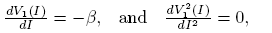
Forecasting the evolution of an infectious disease has been the main motivation for the construction of mathematical epidemiological models. This is because knowing the evolution of the infectious disease allows the design of public health strategies to control or eradicate the disease. In this sense, it is essential to know the existence of threshold values that predict whether the disease will be spread or if it can be controlled. Classically, the basic reproduction number, denoted by R 0, is a threshold value that can describe two scenarios: a disease is persistent if R 0 is greater than one, and it dies out if R 0 is smaller than one. R 0 can be defined as the expected average number of new infected individuals produced by a single infective individual, in a completely susceptible population, during its infective period. For those reasons, R 0 can be associated to a forward bifurcation in R 0 = 1. In that case, the endemic equilibrium exists only for R 0 > 1. Then, there is not an endemic state when R 0 < 1 (see Figure 1). In recent years, backward bifurcation phenomenon has attracted interest in mathematical epidemiology (see Figure 2). This is due to the fact than when a backward bifurcation appears, reducing R 0 below 1 would not eradicate the disease, if the initial infective population size is sufficiently large. In this case, a bistability phenomenon occurs when R 0 is less than 1. There will be two locally asymptotically stable equilibrium points, one with no disease (disease-free equilibrium) and other one with a positive endemic level. In order to eradicate the disease, one must further reduce R 0 so far that it passes a so-called saddle-node bifurcation that exists for values of R 0 < 1 and enters into the region where no endemic equilibrium points exist. In that case, the disease-free equilibrium is globally asymptotically stable (see Figure 2 A)). The basic reproduction number does not provide a description of the necessary elimination effort; rather the description of the effort is provided through the value of the critical parameter at the turning point. Furthermore, if a backward bifurcation appears in R 0 = 1, then an (stable) endemic equilibrium exists for R 0 just above 1. This endemic state has a large infectious population. So the result of R 0 rising above 1 would be a sudden and dramatic jump in the number of infectious individuals. (see Figure 2 A)). In contrast, a backward bifurcation can exist when R 0 is bigger than 1. This bifurcation emerges from an endemic state that is an equilibrium point which belongs to a forward bifurcation. This forward bifurcation emerges from the disease-free equilibrium when R 0 = 1. In this scenario, a bistability phenomenon can occur in a neighborhood of R 0 = 1 in two ways. There will be either two locally asymptotically stable equilibrium points, one with no disease and other with a positive endemic level for R 0 < 1 (see Figure 2 B)), or two locally asymptotically stable endemic equilibrium points for R 0 > 1 (see Figure 2 C)). Thus, it is important to identify backward bifurcation in order to obtain thresholds for the disease control. Again, in order to eradicate the disease, one must further reduce R 0 until it passes a so-called saddle-node bifurcation that exists for values of R 0 < 1 and enters into the region where no endemic equilibrium points exist. In such case the disease-free equilibrium is globally asymptotically stable. To sum up, the bistability phenomenon may be due to either a backward bifurcation in the disease-free equilibrium (see Figure 2 A)) or a backward bifurcation in an endemic equilibrium (see Figure 2 B) and C)).
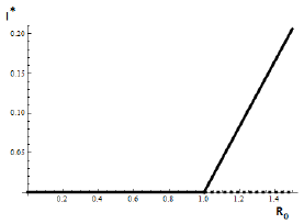
Figure 1 Forward bifucation in R 0 = 1. In this case, the strategy of carrying R 0 below one is enough to eradicate the infectious disease.
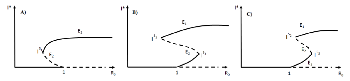
Models with backward bifurcations have been studied in an epidemiological context. For example, in generic compartmental models [2], [15], [18], [20], in models describing the spread of specific diseases like tuberculosis [12], dengue [1], [2] and sexually transmitted diseases [4], [5], [13]. Also, vaccine-preventable diseases [2], [4], [6], [7], [14], [16], and the acquired immunity is a debated cause for its occurrence [11]. There can be no doubt that existence of a backward bifurcation can be associated with nonlinear forces of infection [4], [10] or treatment rates of the disease [17]. However, in each epidemic model analyzed in literature, if a backward bifurcation appears, the origin of the backward bifurcation is unique. That is, a backward bifurcation might emerge from either the disease-free equilibrium when R 0 = 1 (see Figure 2 A)) or from an endemic state for R 0 > 1 (see Figure 2 B) and C)).
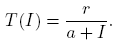
On the other hand, in the literature many forms of the per-capita treatment function T (I) appears, for example,  or piecewise linear functions for the treatment rate (see [3], [8], [9], [17], [18], [19], [21]).
Particularly, Zheng et al. [21], analyzed an SIR model with a per-capita treatment rate given by
 (1)
(1)
They proved the existence of a backward bifurcation in the disease-free equilibrium point and bistability phenomenon for some conditions over the parameters as it is shown in the Figure 2 A).
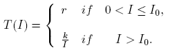
Meanwhile, Wang [18], analyzed an SIR model with a per-capita treatment rate given by
 (2)
(2)
The author proved the existence of a backward bifurcation in a non trivial equilibrium point and the bistability phenomenon for some values on the parameters in a neighborhood of R 0 < 1, as is shown in Figure 2B).
Observe that, in each case showed above, the derivative of the per-capita treatment rate T (I) is different. This observation leads us to assume that the velocity (shape) of the percapita treatment rate may explain the nature of the point where a backward bifurcation emerges. That is, if the backward bifurcation comes from either a trivial equilibrium point or from a non trivial equilibrium point.
In this work we present an SIR model which describes an infectious curable disease and a per-capita treatment rate given by 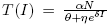 , where δ is a density-dependent factor of the treatment. This election of the treatment rate catches the impact of the infection in the treatment. Particularly, for some values on the parameters, the model shows a bistability phenomenon, which is associated to either the existence of a backward bifurcation, in the trivial equilibrium point, when R
0 = 1, or to the existence of a backward bifurcation, in an endemic equilibrium point, when R
0 > 1. That is, there are stable endemic states in a neighborhood of R
0 = 1. In summary, this election of T (I) captures two possible scenarios for the existence of a backward bifurcation in function of the velocity of the per-capita rate for some values of the model parameters.
, where δ is a density-dependent factor of the treatment. This election of the treatment rate catches the impact of the infection in the treatment. Particularly, for some values on the parameters, the model shows a bistability phenomenon, which is associated to either the existence of a backward bifurcation, in the trivial equilibrium point, when R
0 = 1, or to the existence of a backward bifurcation, in an endemic equilibrium point, when R
0 > 1. That is, there are stable endemic states in a neighborhood of R
0 = 1. In summary, this election of T (I) captures two possible scenarios for the existence of a backward bifurcation in function of the velocity of the per-capita rate for some values of the model parameters.
The structure of the work is described as follows: in section 2 we introduce the model and calculate its basic reproductive number R 0. In section 3 the direction of the bifurcation in R 0 = 1 is analyzed. Furthermore, existence of multiple steady states for R 0 < 1 as well as for R 0 > 1 are shown. From here, it will be possible to find threshold values for existence of equilibrium points and a criterion of stability of the equilibrium points is given. Also, in this section, numerical simulations of the results are shown. Finally, in section 4 we present some conclusions and provide an explanation of the results.
2. The model
Let us consider an SIR model: Let N(t) be the total population. The population N(t) is divided into three classes; a susceptible class S(t), an infectious class I(t), and a recovery class R(t). So N(t) = S(t) + I(t) + R(t).
The compartmental epidemic model is given by
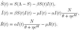 (3)
(3)
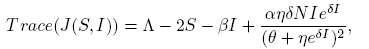
All parameters are positive constants, with the following interpretation; Λ is the carrying capacity in the absence of disease, μ is the birth-death rate, β is the infection coefficient. In the per-capita treatment rate,  , α is the treatment rate, δ is a densitydependent factor for the treatment. Furthermore, η and θ measure the extent of the effect for the infectious being delayed because of the treatment. In this case, the per-capita treatment rate T (I) has an unique inflection point in
  . Note that for values of I < I* the function is concave and for values of I > I* the function is convex.
Note that  is the average number of infectious individuals where the velocity of the per-capita treatment rate has a maximum, and in this point the response of the strategy changes velocity. This changes may be due to numerous factors involving treatments, for example, number of hospitals, number of doctors or nurses, cost of public health policies, etc. This critical value of I can be related to the maximum value of the total treatment rate,
 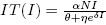 .
.
Before going into further detail, we simplify the model. Since the first two equations of (3) are independent of the third one and their dynamic behavior is trivial when I(0) = 0 for t > 0, it suffices to consider the first two equations with I > 0, which are independent of R(t).
Thus, we restrict our attention to the following reduced model:
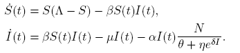 (4)
(4)
It is easy to verify that model (4) admits the equilibria Ee = (0, 0) and E 0 = (Λ, 0). The Jacobian matrix associated to model (4) is given by
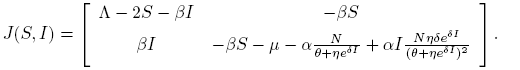 (5)
(5)
The Jacobian matrix (5) evaluated in the trivial equilibrium point Ee (which is the extinction scenario) is given by
 (6)
(6)
So, the eigenvalues associated to (6) are λ
1 = Λ and 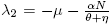 . The equilibrium Ee
is always unstable for all values of the parameters. This result is consistent with the fact that there is a constant recruitment rate in the model proposed.
. The equilibrium Ee
is always unstable for all values of the parameters. This result is consistent with the fact that there is a constant recruitment rate in the model proposed.
Now, the Jacobian matrix (5) evaluated in the disease-free equilibrium point, E 0, is
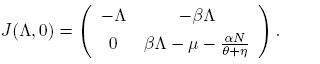 (7)
(7)
So, the eigenvalues associated to (7) are λ
1 = −Λ and 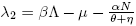 .
.
The basic reproductive number is defined as 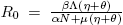 . Observe that R
0 is independent of the dense-dependent factor, δ. From our previous discussion we arrive to the following result.
. Observe that R
0 is independent of the dense-dependent factor, δ. From our previous discussion we arrive to the following result.
Lemma 2.1. The equilibrium point E 0 is locally asymptotically stable if and only if R 0 < 1.
The next step is to investigate the nature of the direction of the bifurcation in the trivial equilibrium E 0 when R 0 = 1. To do this, we will use Theorem 1 in [12], which is based on the use of the center manifold theory.
3. Endemic equilibria and bifurcations
3.1. Direction of the bifurcation
Let a and b be the coefficients of the normal form representing the dynamics of the system in the central manifold. Theorem 1 in [12], describes the role of such coefficients in deciding the direction of the transcritical bifurcation occurring at Φ = 0.
We apply Theorem 1 to describe the direction of the bifurcation at R
0 = 1 associated to system (4) in the trivial equilibrium E
0. Let us define 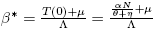 , such that R
0(β*) = 1, which is denoted by R*
0.
, such that R
0(β*) = 1, which is denoted by R*
0.
Observe that the eigenvalues of the matrix
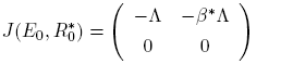 (8)
(8)
are given by λ 1 = −Λ and λ 2 = 0.
Thus, λ 2 = 0 is a simple zero eigenvalue and the other eigenvalue is real and negative. Hence, when R 0 = R* 0 the disease-free equilibrium E 0 is a non hyperbolic equilibrium: the assumption (A1) of Theorem 1 in [12] is then verified.
The right eigenvector associated with the zero eigenvalue λ 2 is given by w = [−β*, 1], and the left eigenvector associated to the zero eigenvalue λ 2 is given by v = [0, 1]. Observe that v · w = 1. The coefficients a and b defined in the Theorem 1 are
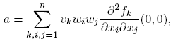 (9)
(9)
 (10)
(10)
Computing explicitly taking into account the system (4), it follows that:
 (11)
(11)
and
 (12)
(12)
The coefficient b = Λ is always positive, so that, according to Theorem 1 [12], the local dynamics around the disease-free equilibrium for R* 0 is determined by the sign of the coefficient a. As a consequence, the following condition ensures the occurrence of a backward bifurcation at R 0 = R* 0:
 (13)
(13)
If the inequality (13) is reversed,
 (14)
(14)
a forward bifurcation at R 0 = R* 0 is followed.
All these considerations allow us to state the following lemma:
Lemma 3.1. Let R* 0 be:
Next, existence of endemic equilibrium points is showed.
3.2. Existence of endemic equilibria
The nullclines of system (4) are given by
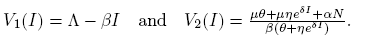 (15)
(15)
Note that V
1(0) = Λ and  . Also, R
0 > 1 if and only if V
1(0) > V
2(0). And
. Also, R
0 > 1 if and only if V
1(0) > V
2(0). And 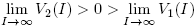 .
.
Deriving twice the nullclines we have
 (16)
(16)
and
 (17)
(17)
Observe that V
1(I) and V
2(I) are decreasing functions for all values of I for δ > 0. Also,  is an inflection point of V
2(I). We defined this value of I as
is an inflection point of V
2(I). We defined this value of I as  .
.
Note that if δ < 0, then an unique equilibrium point exists. This case is related to a forward bifurcation in R 0 = 1.
Lemma 3.2.
Let 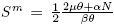 , δ > 0, θ > η. If
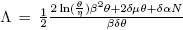 , then (Im, Sm
) is an equilibrium point of the system (4).
, then (Im, Sm
) is an equilibrium point of the system (4).
Lemma 3.3. Let (Im, Sm ) be an equilibrium point of system (4).
Proof. The derivatives of the nullclines evaluated in the inflection point are given by
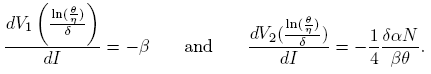
Thus, the slope at the inflection point in the nullcline V 2 is greater than the slope at the inflection point of the nullcline V 1 if 4β 2 θ > δαN; then, nullclines intersect transversely and V 2(I) > V 1(I) in a neighborhood of the inflection point, which is a coordinate of the equilibrium point. On the other hand, V 1(0) > V 2(0) if and only if R 0 > 1. By continuity of V 1(I) and V 2(I), the system (4) has three equilibrium points if R 0 > 1, and two equilibrium points if R 0 < 1. ☑
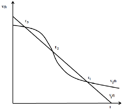
Figure 3 Nullclines of the system (4) in the case where three equilibria points exist. There exists a forward bifurcation emerging from the disease-free equilibrium in R 0 = 1 and a backward bifurcation arising from an endemic equilibrium for values of R 0 > 1. This results are due to the continuity of the functions as function of the model parameters.
Case i) is shown in Figure (3).
We can summarize the above results in the following theorem.
Theorem 3.4. For the model (4). Let (Im , Sm ) be an equilibrium point of the system (4).
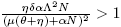
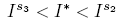
a) If and R
0 < 1, there is a saddle equilibrium point, which bifurcates into two positive equilibrium points (Backward Bifurcation on the trivial equilibrium (seeFigure 2 A))).
and R
0 < 1, there is a saddle equilibrium point, which bifurcates into two positive equilibrium points (Backward Bifurcation on the trivial equilibrium (seeFigure 2 A))).
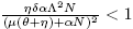
b) If and R
0 > 1, there are two saddle equilibrium points which bifurcate into two positive equilibrium points each one (Backward Bifurcation on the non trivial equilibrium, seeFigure 2 B) and C)).
and R
0 > 1, there are two saddle equilibrium points which bifurcate into two positive equilibrium points each one (Backward Bifurcation on the non trivial equilibrium, seeFigure 2 B) and C)).
Observing Figure (2) we can conclude that there are saddle equilibrium points associated to system (4). This cases are analyzed in what follows.
First, note that points on the nullclines, where the nullclines have the same derivatives, satisfy the equation
 (18)
(18)
where y = eδI , A = β 2 η 2, B = 2β 2 θη − ηδαN and C = β 2 θ 2.
The solutions of the equation (18) are given by
 (19)
(19)
where ρ = αδN(αδN − 4β 2 θ).
Observe that ρ > 0 if 4β 2 θ < αδN, ρ = 0 if 4β 2 θ = δαN and ρ < 0 if 4β 2 θ > δαN. So, we have the following results about saddle points of the system.
Lemma 3.5. For system (4):
a) If ρ > 0, there are two values I where the nullclines have the same derivative.
b) If ρ = 0, there exists a unique value I where the nullclines have the same derivative.
c) If ρ < 0, there are not values I where the nullclines have the same derivative.
Lemma 3.6. For system (4):
a) is an equilibrium point of the model (4) if and only if
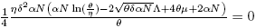 and ρ = 0.
b)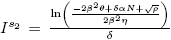 and
and are equilibrium points of the model (4) if and only if
 and ρ > 0.
In the next section we will deal with the stability of these equilibria.
3.3. Stability analysis
The criterion of determinant and trace is used to find conditions over the stability of the equilibrium points.
The Jacobian matrix (5) evaluated in the equilibrium point (S*, I*) is given by
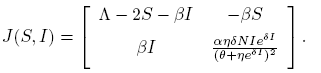 (20)
(20)
Note that
 (21)
(21)
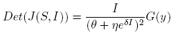
and
 (22)
(22)
where G(y) = (A 1 y 2 + B 1 y + C 1), y = eδI , A 1 = β 2 η 2 S, B 1 = η(2β 2 θS + αδΛN − 2αδNS − αδβNI) and C 1 = β 2 θ 2 S.
Observe that G(0) > 0 and  .
.
Particularly, Det(J(Is 1 )) = Det(J(Is 2 ))) = Det(J(Is 3 )) = 0 can be proved. So, there exists values of
such that Det(J(I*)) < 0. On the other hand, if the Trace(J(S*, I*)) is analyzed, the following result can be written using the Trace-Determinant criterion using the definitions of Is 1 , Is 2 and Is 3 as in Lemma 3.6.
Lemma 3.7.
If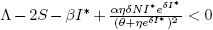 and I* < Is
3
or I* > Is
2
, the equilibrium point (I*, S*) is locally asymptotically stable.
and I* < Is
3
or I* > Is
2
, the equilibrium point (I*, S*) is locally asymptotically stable.
On the other hand,
Lemma 3.8. If Is 3 < I < Is 2 , then the non trivial equilibrium point (I*, S*) is unstable.
An analogous analysis can obtained for Is 1 defined in Lemma 3.6.
Lemma 3.9.
If and I* > Is
1
the equilibrium point (I*, S*) is locally asymptotically stable.
and I* > Is
1
the equilibrium point (I*, S*) is locally asymptotically stable.
3.4. Simulations
In this section, we present some numerical simulations using XPPAUT 7.0 and Mathematica 11 to show different bifurcation diagrams and phase portraits corresponding to distinct treatment scenarios for the system 3. Also, The bifurcation diagram associated to simulations illustrates the bifurcation to multiple equilibria. Simulations show existence of a backward bifurcation emerging from either the disease-free equilibrium point when R 0 = 1, or from an endemic equilibrium point when R 0 > 1 (see Figure 2).
For the case where there are two endemic equilibrium points (backward bifurcation), typical dynamical behavior is the following: the stable manifolds of the saddle point E 2 split the feasible region in two parts. Positive orbits in the lower part approach to trivial equilibrium point E 0 and positive orbits in the upper part approach to endemic equilibrium point E 1. So, the model shows a bistability phenomenon for values of R 0 < 1 (see Figure 4 B)).
On the other hand, if three endemic equilibrium points exist, the model shows a forward bifurcation in R 0 = 1, and a backward bifurcation in an endemic equilibrium for R 0 > 1. In this case, for different values of the parameters the model can show two different scenarios.
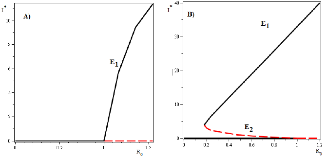
Figure 4 A) Forward bifurcation with δ = −0.1027 < 0. In this case, condition (14) is satisfied. Other values of the parameters are given by; β = 0.0099, θ = 2000, η = 2.5, α = 0.1,N = 100, μ = 0.001, Λ ∊ (0.0605, 1.5), > 1. B) Backward bifurcation in R0 = 1 and the values of the parameters are given by; β = 0.0246, θ = 0.001, η = 0.1, δ = 0.9, α = 0.001,N = 2, μ = 0.001, Λ = (0.152, 1.014), < 1 and .
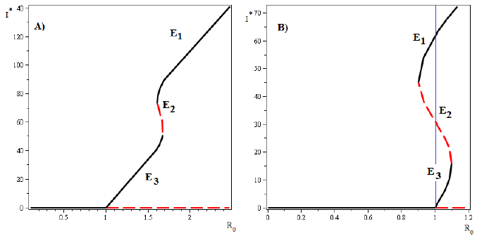
Figure 5 A) Bistability phenomenon for values of R 0 > 1 and a forward bifurcation in R 0 = 1. The values of the parameters in this case are: β = 0.0099, θ = 2000, η = 2.5, δ = 0.1027, α = 0.1,N = 100, μ = 0.001, Λ ∊ (0.0605, 1.5), > 1 and . B) Bistability phenomenon for values of R 0 < 1 and forward bifurcation in R 0 = 1. The values of the parameter are given by: β = 0.2317, θ = 0.22, η = 0.01, δ = 0.1, α = 0.1,N = 8, μ = 0.001, Λ ∊ (0.5630012132, 0.66579), = .066405969 and = 0.3203519571.
In the first scenario, the saddle point Is 2 appears when R 0 is bigger than 1. In this case, the stable manifold of the saddle point E 2 split the feasible region in two parts. Positive orbits in the lower part approach the endemic equilibrium point E 3 and positive orbits in the upper part approach the endemic equilibrium point E 1, which only exist for values of R 0 > 1. In the second scenario, the saddle point Is 2 appears when R 0 is less than 1. In this case, the stable manifold of the saddle point E 2 splits the feasible region in two parts: positive orbits in the lower part approach either the endemic equilibrium point E 3 or disease-free equilibrium point E 0, and positive orbits in the upper part approach the endemic equilibrium E 1, which exists for values of R 0 < 1 as well as for values of R 0 > 1. (see Figure 5 B)). The phase portrait and the vector field of directions around the fixed equilibria for both cases are shown in Figure 6.
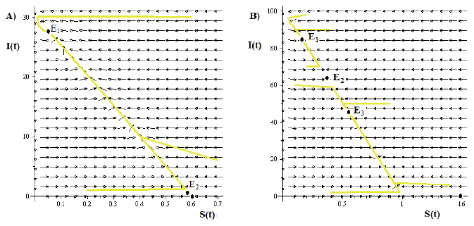
Figure 6 A) Typical dynamics for the solutions in the portrait phase when the model (4) has a backward bifurcation in R 0 = 1 and bistability for R 0 < 1. Whereas that, Case B) shows the typical dynamics for the model (4) for a bistability phenomenon, for values of R 0 > 1 and a forward bifurcation in R 0 = 1.
4. Conclusions
In this paper we have considered an SIR epidemic model, which incorporates a percapita treatment function T (I). This model exhibits a backward bifurcation emerging from either a disease-free equilibrium point or from an endemic equilibrium point when some conditions over the parameters are satisfied. For some values of the parameters, in the two previous cases, a bistability phenomenon occurs. Particularly, observe that, when T (I) is an increasing function (this is the case when δ < 0), the forward bifurcation occurs independently of the values of the other parameters, and existence of a backward bifurcation is excluded (see Figure 4 A)). On the other hand, if the per-capita treatment rate, T (I), is a monotone decreasing function (δ > 0), then the model (4) exhibits two possible scenarios with a backward bifurcation for some values of the parameters. First scenario is a backward bifurcation arising from the disease-free equilibrium (R 0 = 1) (see Figure 4 B)). The second case is associated to a forward bifurcation in R 0 = 1 and a backward bifurcation emerging from an endemic equilibrium point for R 0 > 1 (see Figure 5 A) and B)).
The biological consequences of this result are far-reaching, since it shows that a way to avoid the undesirable bistability phenomenon is applying an efficient and effective treatment (δ < 0), specially for those diseases that respond to treatment and for which there is no spontaneous recovery, that means, it is sufficient take an unbounded total treatment rate. This means, the total treatment rate, IT (I), does not have a maximum. Otherwise, if an inefficient treatment strategy is applied (the total treatment rate reaches its maximum and decreases), multiple endemic states could appear together with a bistability phenomenon. From here it follows that if the treatment application was inefficient from the beginning, improving it can worsen the epidemic outbreak. Since in this case there would be a point of inflection that could generate the existence of three endemic equilibrium states. That is, the model suggests that applying the treatment inefficiently forever and carrying R0 below the saddle point would lead solutions to disease-free equilibrium. An important consequence of the results is the following: an epidemic control strategy associated to a forward bifurcation in R 0 = 1 can be worse that the control strategy associated to a backward bifurcation in R 0 = 1. This is due to the endemic equilibrium point E 1 in the first scenario may be bigger than E 1 in the second when R 0 is less than 1. Hence, it is very important to understand the mechanisms that can induce this peculiar bifurcation and its point of origin.
In further work, existence of a Hopf bifurcation as function of the total treatment rate, IT (I), will be analyzed. Particularly, when IT (I) has a maximum value.

