


 Inglés (pdf)
 Articulo en XML
 Referencias del artículo
 Enviar articulo por email
 Citado por SciELO
  Citado por Google
  Similares en
SciELO
Similares en
SciELO  Similares en Google
 Permalink
1. Introduction
A class of models that appears naturally in a wide number of phenomena are the random differential equations. This occurs because randomness is a powerful tool and concept to control complex systems involving a large number of variables and particles. The basic idea is to describe complex systems by means of their statistical properties. Another kind of phenomena are those governed by quantum mechanics and the uncertainty principle. In this direction, we have Schrödinger equations, and their random versions, which are the core in the study of condensed matter.
The semilinear Schrödinger equation reads as

where
 is the Planck constant and i is the imaginary unit. When looking for standing wave solutions, namely those with the special form
 we are leading to solve an equation of the type

From the physical viewpoint, the function V is the potential energy, and therefore the force acting on the system is given by F(x) = - ∇V(x). In [20] the author considered a singularly perturbed version and obtained the existence of solution by assuming that V is such that
In [8], the authors showed that the same holds if V has a local minimum. Later, many authors considered multiplicity and qualitative properties of solutions (see [1], [2] and references therein).
The main interest of this paper is to study situations where the potential V is not deterministic. We show existence and probabilistic properties for a nonhomogeneous random version of (2), namely
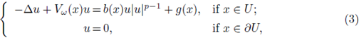
where 1 < p < ∞,Vw is a random variable
 is a bounded domain and the terms b, g ∈ L∞( (U) are deterministic. In the case V ≡ 0 Pohozaev-type identities provide non-existence of positive solutions for (2) with critical and supercritical variational values
 So, it is natural to consider a nonhomogeneous term on the right-hand side of (3). Here we desire to cover not only high-powers for p, but also the effect on the random term Vw. Our results work well for b ≡ 1, and in this case (3) is precisely the perturbation of (2) by the non-homogeneous term g. Also, the boundedness of U, b, g are not essential and could be circumvented by working in other settings, such as homogeneous weighted L∞-spaces, PMa-spaces and anisotropic Lebesgue spaces (see, e.g., [11], [12], [13], [14], [15]). However, here this condition will simplify matters a bit. The random potential Vw is constructed as follows: given a continuous function
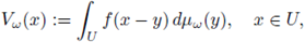
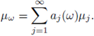
 we consider

where μw is a M(U)-valued random variable and M(U) denotes the set of all Radon measures on U with finite variation.
We present here some examples of (4) that have been treated in the literature (see e.g. the review [18]). We first consider a model of an unordered alloy, that is, a mixture of several materials with atoms located at lattice positions. Assuming that the type of atom at the lattice
 is random, we are led to consider potentials of the type

where the random variables qi describe the charge of the atom at the position i of the lattice. Other examples can be obtained by considering materials like glass or rubber, where the position of the atoms of the material are located at random points ηi in space. By normalizing the charge of the atoms, the suggested potential is formally

where the
 are random variables which localize the atoms in space.
The class of potentials allowed here is sufficiently large to consider many known models. For example, the case of glass considered in (6) can be obtained by taking the random point measure
 Actually, for this choice of the measure we have that

Also, a combination of potentials like (5) and (6), namely
is also covered by (4) with
 It is not difficult to see that we can also consider other models like, e.g., the Poisson model (see [18] for more examples).
The models (5) and (6) correspond to discrete measures µw for which results about localization, spectral properties and decays can be found in [18], [21]. For Schrödinger equations defined in a lattice, i.e.
 we refer the reader to [5]. Considering a random time-dependent potential for (1), the authors of [3] studied asymptotic behavior of solutions by showing convergence for Gaussian limits when the two-point correlation function of the potential is rapidly decaying. Still for time-dependent random potentials, scaling limits for parabolic waves in random media were investigated in [10]. Another type of random equations are the parabolic ones, for which we refer to the works [4], [6], [7] and their references. In fact, the authors of [4] extended regularity properties (Kalita's results) to the stochastic case by considering quasilinear parabolic systems under a random perturbation of Itô type (see [16] for further results on stochastic PDEs).
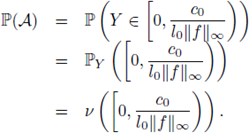
In this paper we show that a solution for the nonlinear elliptic PDE (3) exists almost surely (or not) depending on the v-measure of the interval
 where v is the probability measure induced on
 by the random variable
 and k0 is a given constant (see Theorem 3.2). For that, we obtain Proposition 3.1 which seems not to be available in the literature even for the deterministic version of (3). Solutions are understood in an integral sense based on Green functions. In Remark 3.3 and Corollary 3.4, we give some examples of continuum random potentials covered by our results. Since we are considering L∞-valued random solutions, it is natural to ask about the expected value of the L∞-norm of solutions. In Theorem 3.5, we provide an estimate for this value depending on the size of the potential. Moreover, we obtain a law of larger numbers for solutions obtained by independent ensembles. It is worth to mention that, when dealing with the random variable
 that maps an element of Ω in the solution of (3) associated with the random potential Vw, we need to consider some known concepts of real random variables in a more general setting (see Section 2 for more details).
As a further comment, we observe that the random potentials considered here are built from a very general probability space. In this setting it does not always make sense to ask what is the probability that the problem (3) has a solution in L∞(U). In order to give some sense to this question we should restrict ourself to probability spaces
 and random potentials V where the set

is an event (measurable). Working in such probability spaces, Theorem 3.2 gives us immediately a lower bound for the probability of the non-linear problem (3) having a solution.
The manuscript is organized as follows. In the next section, we introduce some notations, basic definitions and give some properties for an integral operator associated with the random potential Vw - The main results are stated and proved in Section 3.
2. Preliminaries and notation
Throughout this paper
denotes a given complete probability space. If  is a measurable space, any
 measurable function X : Ω → E will be called a E-valued random variable. We use the abbreviation a.s. for almost surely or almost sure.
Let
 be a bounded domain. We adopt the standard notation M(U) to denote the set of all Random measures on U with finite variation and we call
 the σ-algebra of the borelians of M(U) generated by the total variation norm. The space of all bounded continuous real-valued functions defined on U will be denoted by BC(U). Since BC(U) is a metric space with the supremum norm, when we refer to a BC(U)-valued random variable, the considered σ-algebra is always the one generated by the borelians. Similarly to a X-valued Borel random variable X : Ω → X, where X is an arbitrary metric space.
The random potentials considered here are the BC(U)-valued random variables defined as follows. Take any random variable X : Ω → M(U) (which is simply a random measure in M(U)) and a fixed function
 Then, for μ
ω
= X(ω), the function V : Ω → BC(U) defined by
Then, for μ
ω
= X(ω), the function V : Ω → BC(U) defined by
is a BC(U)-valued random variable that will be called a random potential. To see that V is a well-defined BC(U)-valued random variable, is enough to consider the mapping Tf: M(U) → BC(U) given by
and to observe that V = T¡ o X. In fact, if we denote by
 the total variation of the measure μ, we have the inequality

which implies that Tf (μ) belongs to L∞(U). Also, proceeding as in (8) and using dominated convergence theorem, one can show that T f(μ) is a continuous function, and so Borel measurable. It follows that V is a composition of two Borel measurable functions and a BC(U)-valued random variable.
Let
 be a measure space. For a measurable function f we define

and the space
 as the set

When dμ = dx is the Lebesgue measure in
 we simply denote
 Although we are assuming that
 most of the results presented here are also valid if we suppose only the weaker condition

In order to state some convergence results, we need to use the notion of Bochner integrals. Let
 be a Banach space and
 be a probability space. If
 is a X-valued Borel random variable such that X = Y a.s. in Ω, where Y: Ω → X is a X-valued Borel random variable with Y(Ω) ⊂ X separable, and
then there exists a unique element
 with the property
for all
 where X* stands for the dual of X. Following the standard notation, we write
We call
 the Bochner integral of X with respect to
 More details about the existence and some properties of this integral can be found in [17], [19].
For X-valued random variables, we define the convergence in probability similarly to the real-valued case. If {Xj} is a sequence of X-valued random variable, we say that X j converges to a X-valued random variable X in probability if for all ε > 0, we have

When X is a real-valued random variable, we use the usual notation and denote the expected value of X and its variance by

respectively. For both senses of expectation presented above, we also use the notation

when A ⊂ Ω is measurable and the right-hand-side of (10) makes sense.
Let X and Y be two E-valued random variable in the same probability space. We say that they are identically distributed if for all
 we have
Now we introduce the notion of independence. Given a finite set of random variables X1,... Xj, they are said to be independent if for all
 we have
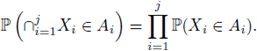
Finally, a sequence of random variables {X1, X2,...} is independent if all finite collection of this sequence form a set of independent random variables.
3. Main results and proofs
Let G be the Green function of the Laplacian operator -Δ in the bounded domain
 with n ≥ 3. It is known that (see [9]), for all x, y ∈ U, there holds
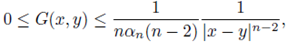
where α
n
stands for the volume of the unit ball in
 Hence, if we denote by dU the diameter of U, namely
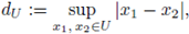
and

a straightforward calculation provides
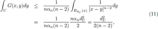
for all x ∈ U. From now on, we write only l 0 = l 0(n,U) to denote the quantity
Inequality (11) implies that the map H : L∞(U) → L∞(U) given by
is well-defined. More specifically, for any ϕ ∈ L∞(U), we have that
and then

Standard calculations show that the problem (3) is formally equivalent to the integral equation

A solution of (14) is called an integral solution of (3).
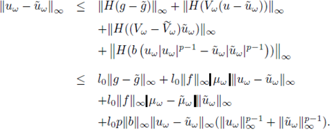
In what follows, we give estimates for the terms of (14) in order to apply a fixed point argument. We first set X := L∞(U) and define, for any fixed ω ∈ Ω, the linear function T : X → X given by

It follows from (13) and (8) that, for any u G X, there holds

and so
For the nonlinear term in (14), we define B : X → X by

For
 there holds

and then it follows that

This inequality and the same argument used in (15) imply that

for any
All together, the above estimates enable us to solve the random equation (3) as follows.
Proposition 3.1. Given f, b, g ∈ L∞ (U) and w ∈ Ω, we consider the potential V w induced by the random measure µw: = X(w). Let l0 be the quantity introduced in (12) and set

If ε > 0 and w ∈ Ω are such that

and
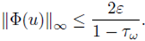
 then the equation (3) has a unique integral solution uw (i.e. it satisfies (14)) such that

Proof. For each ε > 0 and ω ∈ Ω satisfying (18), we consider the closed ball
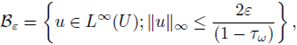
endowed with the metric
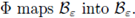
 We are going to show that the map

is a contraction on the complete metric space
 Using the estimates (13), (15), and (16) with
 we obtain
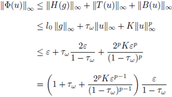
for all u Hence, it follows from (18) that
This shows that
 .
.
For all
 it follows from (15) and (16) that
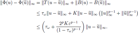
In view of (18), the above estimate implies that Φ is a contraction in
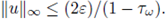
 Now, the Banach fixed point theorem assures that there is a unique solution u for the integral equation (14) such that
The next results are related to the randomness introduced by the random potential V and existence of solutions for the problem (3). Roughly speaking, we first obtain the probability of (3) having a solution via the method discussed above. In the sequel we discuss a law of large numbers for a sequence of random potentials.
Theorem 3.2. Let v be the probability measure induced on
 by the random variable
 Let g ∈ L
∞
(U) be such that
Let g ∈ L
∞
(U) be such that
 where
where
 Choose 0 < c0 < 1 in such a way that
 with
with
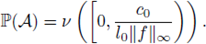
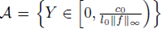
Let A be the set of ω ∈ Ω such that (3) has a solution u(·, ω) given by Proposition 3.1 with ε = ε 0 . The set A is called the admissible one for the random variable X(ω) and non-homogeneous term g.
(i) The set A is F-measurable, and the probability of (3) having a solution is
(ii) Let
 be two solutions of (3) corresponding, respectively, to
 and
and
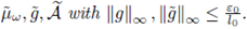 Assume that
 and define

We have that
for all

(iii) The map U : A → L∞ (U) given by U(ω) := u(·, ω) is a random variable, and there holds
for all ω ∈ A.
Proof. We first notice that ω ∈ A if only if
 verifies with ε = ε0
. Then, if
verifies with ε = ε0
. Then, if
 it follows that
 is measurable and
This establishes (i).
Now we deal with item (ii). Firstly, observe that
 where
where

Subtracting the integral equations verified by u
w
and
 and afterwards computing
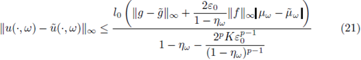
 we obtain
It follows from (19) that

The two above expressions give us
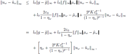
which yields (21).
Taking
 independent of w, i.e. μ
w
= μ and
independent of w, i.e. μ
w
= μ and
 for all ω ∈ Ω, we can see from (17) and (21) that the data-map solution
 is continuous from

where u is the deterministic solution of (3) corresponding to the data (µ, g). From this, and because
 given by
 is measurable, it follows that the composition
 is measurable.
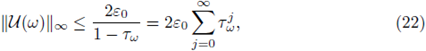
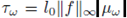
In view of the series
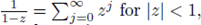 we finish by observing that (22) follows from (19) with ε = ε0 and ω ∈ A.
Remark 3.3. Here we give examples of random potentials for which there exists a solution almost surely in Ω. The first occurs if we suppose that the measure v has compact support contained in the interval [0,a], with
 In this case it follows from item (i) of Theorem 3.2 that
 i.e., the solution exists almost surely in Ω. Second, take a sequence
 in M(U), and let
 be a sequence of random variables from 0 to R. Consider the random variable µ
w
defined by
be a sequence of random variables from 0 to R. Consider the random variable µ
w
defined by
For some q > 1, suppose that
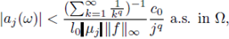
for all
 Then,
Then,
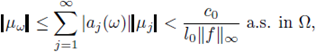
and Theorem 3.2 assures that there is an integral solution for (3) a.s. in Ω.
In the sequel we show how the Borel-Cantelli's Lemma can be used to give a sufficient condition for the existence of solution a.s. in Ω.
Corollary 3.4. Let c
0
and g be as in Theorem 3.2. Let
 be a sequence in M(U) and let
 be a sequence of random variables from Ω to
 Assume that the series
is convergent in M(U).
For each
 define
and
 If
If
then there is an integral solution for (3) almost surely in Ω .
Proof. By Borel-Cantelli's Lemma we get that
 that is,
It follows that, for almost sure ω ∈ Ω, there is j0 = j0(w) such that for all j > j0, we have

Therefore, by taking the limit as j → ∞, we obtain
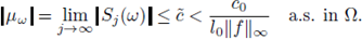
This inequality and Theorem 3.2 imply that there is an integral solution u(x,w) for (3) almost surely in Ω.
A straightforward calculation shows that in general
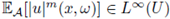
 does not satisfy the equation (3), even if we replace the random potential by its mean. However, we are able to obtain some information on the average and moments of the random solution uw. Let us mention that, when dealing with the random variable ω → uw, the expectation has to be understood in the Bochner sense (see Section 2). Note also that in fact a solution
 of (14) belongs to the separable subspace

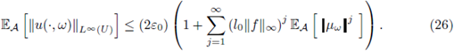
Theorem 3.5. Assume the hypotheses of Theorem 3.2 and denote by u
w
(x) = u(x,w) ∈ L
∞
(U) the solution of (3). Let m ∈
 be fixed and suppose that
Then
 and
and

In the case m = 1, we have
 and
and
Proof. It follows from (22) that

Computing in (27), we obtain
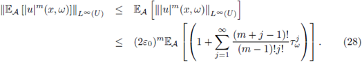
By using the linearity of the expectation and recalling that
 we get the following upper bound for the right hand side of (28):

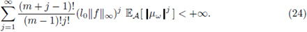
this bound is finite due to (24). From (25) with m =1 and the estimate

we obtain that
 The estimate (26) follows by taking m = 1 in (28)-(29) and afterwards using (30).
In the sequel we show a weak law of large numbers for the random L∞(U)-solutions obtained in Section 2.
Theorem 3.6. Let
 be an independent sequence of random variables X
j: Ω → M(U). Assume that the admissible set A
j = Ω for all j, and let
be an independent sequence of random variables X
j: Ω → M(U). Assume that the admissible set A
j = Ω for all j, and let
 be the solution given by Theorem 3.2 with respect to
 a.s. and

then
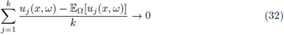
and
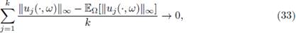
as k → ∞, where the convergences in (32) and (33) are in the sense of probability (see (9)).
Proof. Notice that Xj → X a.s. is equivalent to
 almost surely. From this and the continuity of data-solution map L(·, ·) (see (23)), it follows that

as j → ∞. Recalling (22) and afterwards using (31), we obtain
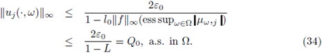
Next, for a fixed g such that
 consider

defined from D to L
∞
(U), where
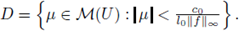 Since Xj's are independent, it follows that
 defined by

are also independent. So, from Chebyshev's inequality, the independence of
 , and (34), we have that
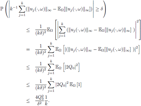
Letting k → +∞ in the above expression, we get (33). The convergence (32) can be proved similarly to (33).


