


 Inglés (pdf)
 Articulo en XML
 Referencias del artículo
 Enviar articulo por email
 Citado por SciELO
  Citado por Google
  Similares en
SciELO
Similares en
SciELO  Similares en Google
 Permalink


1. Introduction
We focus our attention on the following question: Under what growth conditions on f, the nonnegative solutions to the Dirichlet problem will be uniformly bounded? A priori bounds in the L ∞-norm of positive solutions provided a great deal of information, and it is a longstanding open problem.
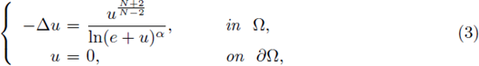
In this paper, we provide sufficient conditions for having a-priori L∞ bounds for a classical positive solutions to the boundary value problem

where Ω ⊂
 N, N > 2, is a bounded C2 domain, and f is a subcritical nonlinearity.
For N = 2, Turner proved the following result. Let Ω be a simply connected domain in R2 with C
2 boundary, let f be a continuous real-valued function on Ω x
, and let us consider

If there are numbers p, A, B > 0 and C ≥ 0 such that 1 < p < 3, and Aup ≤ f (x, u) ≤ max(BCp, Bup) for u ≥ 0, then all such solutions are a priori bounded for some constant C = C(Ω,p, A, B, C). For 1 < p < 2, an analogous result holds when Δ is replaced by a more general elliptic operator. In case of radial symmetry, an analogous result holds for any p > 1, if Aup ≤ f (u) for u ≥ C, and f (u) ≤ max(BDp, Bup) for some D ≥ 0 and all u ≥ 0 (see [27] and also [11, Theorem 1.1]). Brezis and Turner in [4] allow a more general nonlinearity:
 with smaller growth,
 as u → ∞.
When N > 2, the exponent
 of a nonlinearity f(s) = s
2*-1 is critical from the viewpoint of Sobolev embedding; observe that
of a nonlinearity f(s) = s
2*-1 is critical from the viewpoint of Sobolev embedding; observe that
 and the embedding H
1
(Ω) in L* (Ω) is not compact. Pohozaev proved that problem (1) does not have a solution if Ω is starshapped (see [25]), and Bahri-Coron, and Ding proved that problem (1) has a solution if Ω has non trivial topology in a certain sens, including some classes of non star-shaped domains and in particular the case of rings (see [2], [12]).
and the embedding H
1
(Ω) in L* (Ω) is not compact. Pohozaev proved that problem (1) does not have a solution if Ω is starshapped (see [25]), and Bahri-Coron, and Ding proved that problem (1) has a solution if Ω has non trivial topology in a certain sens, including some classes of non star-shaped domains and in particular the case of rings (see [2], [12]).
If
then problem (1) is supercritical. Consider

where B is the unit ball, and
Joseph and Lundgren for balls in
N, N ≥ 3, provided sufficient conditions guaranteeing that (2) has an unbounded sequence of positive solutions (see [19]). Their results are obtained by a careful analysis involving phase plane and qualitative arguments.
If
the problem is of subcritical nature. The discussion given so far suggests that the subcritical growth of / is a necessary condition for the existence of a priori bounds for solutions to (1).
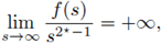
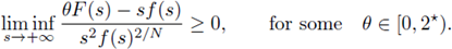
Nussbaum obtain a priori bounds for positive radial solutions in the subcritical radial case, when there exist some δ > 0, s
0 > 0 such that 2NF(s) - (N - 2)sf(s) ≥ δsf(s) for s ≥ s0. Here
 see [23]. Observe that this hypothesis covers the case when
 for some
 Consider f(s) = s
2*-1-ε for ε > 0. It is well known that problem (1) has a solution uε (see P. L. Lions [21] and references therein). Atkinson and Peletier for balls in
3, and Han for the minimum energy solutions in non-spherical domains, proved that there exists x
0 ∈ Q and a sequence uε such that
Consider f(s) = s
2*-1-ε for ε > 0. It is well known that problem (1) has a solution uε (see P. L. Lions [21] and references therein). Atkinson and Peletier for balls in
3, and Han for the minimum energy solutions in non-spherical domains, proved that there exists x
0 ∈ Q and a sequence uε such that
 and
and
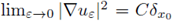 in the sense of distributions, where 6 is the Dirac distribution, and C depends on N and on the best Sobolev constant in
 N (see [1], [18]).
A-priori bounds for subcritical nonlinearities on general domains were raised by Gidas and Spruck in [16] as well as by Figueiredo, Lions and Nussbaum in [11]. The blowup method together with Liouville type theorems for solutions in
N and in the half space
 was introduced by Gidas and Spruck for nonlinearities essentially of the type /(x, s) = h(x)s
p
, with p ∈ (1, 2* - 1) and h(x) continuous and strictly positive. De Figueiredo, Lions and Nussbaum [11] obtained a similar result using a different method. In convex domains in particular, it is based on the monotonicity results by Gidas, Ni and Nirenberg [14], obtained by using the Alexandrov-Serrin moving plane method [26], (which provides a priori bounds in a neighborhood of the boundary), on the Pohozaev identity [25] and on the L
p theory for Laplace equations given by Calderón-Zygmund and Agmon, Douglis and Niremberg estimates (see [17]). They extend some of the results to non-convex smooth domains through the Kelvin transform.
was introduced by Gidas and Spruck for nonlinearities essentially of the type /(x, s) = h(x)s
p
, with p ∈ (1, 2* - 1) and h(x) continuous and strictly positive. De Figueiredo, Lions and Nussbaum [11] obtained a similar result using a different method. In convex domains in particular, it is based on the monotonicity results by Gidas, Ni and Nirenberg [14], obtained by using the Alexandrov-Serrin moving plane method [26], (which provides a priori bounds in a neighborhood of the boundary), on the Pohozaev identity [25] and on the L
p theory for Laplace equations given by Calderón-Zygmund and Agmon, Douglis and Niremberg estimates (see [17]). They extend some of the results to non-convex smooth domains through the Kelvin transform.
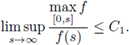
Their results assume on f the following condition:
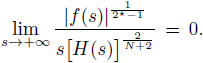
They conjecture that this condition is not necessary, but it is essential in their proof. It can be see n that for f1(s) = s2*-1/ln(s + 2)α with α > 0,

where
 (see [5, Remark 2.3]). We prove the existence of apriori bounds when f (s) = s2*-1/ln(s + 2)α, with α > 2/(N - 2) (see Theorem 1.1).
Next we include several subsections to describe our a priori bounds results on semilinear elliptic equations, and on some non-convex regions. We leave the proofs for the following sections.
1.1. Semilinear elliptic equations
We state the existence of a-priori bounds for classical positive solutions of elliptic equations (1) when
 with
with
 and Ω ⊂
 N is a bounded, convex C
2 domain (see Corollary 2.2 in [5]).
N is a bounded, convex C
2 domain (see Corollary 2.2 in [5]).
Theorem 1.1. Assume that Ω ⊂
N
is a bounded domain with C
2
boundary.
Let us consider the BVP
with α > 2/(N - 2).
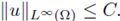
Then, there exists a uniform constant C, depending only on Ω and f, such that for every classical solution u > 0, to (3),
This Theorem is in fact a Corollary of Theorem 2.1 (see Subsection 2.3 for a proof of Theorem 2.1; see also [5, Corollary 2.2]). The ideas of the proof of Theorem 2.1 lie on the following arguments:
Step 1. The moving planes method provides L∞ bounds in a neighborhood of the boundary for classical positive solutions of (1).
Step 2. Pohozaev identity relates some integral defined on Ω with some integral defined on the boundary. This equality, combined with bounds in a neighborhood of the boundary, give us a uniformly bounded integral in Ω.
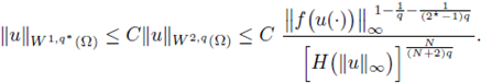
Step 3. The bounded integral in Ω previously obtained through Pohozaev identity, help us in lowering some L
q
(Ω) bound of f(u(·)). Elliptic W
2,q
-regularity with
 and Sobolev embeddings provide us W
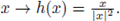
1,q bounds, with q > N. Through Morrey's Theorem, we estimate the radius R of a ball where the function u exceeds half of its L
∞ bound, see fig. 1.
and Sobolev embeddings provide us W
1,q bounds, with q > N. Through Morrey's Theorem, we estimate the radius R of a ball where the function u exceeds half of its L
∞ bound, see fig. 1.
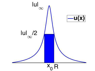
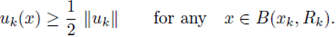
Figure 1 A solution u of (1), its L∞ norm, and the estimate of the radius R such that
 for all x ∈ B(x0,R), where x0 is such that
Step 4. We reason by contradiction assuming that there exists an unbounded sequence of solutions {wfc}. Elliptic W
2,q
-regularity with
 and Sobolev embeddings provide us W1,q bounds with q > N, depending on k.
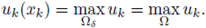
Step 5. Through Morrey's Theorem, we estimate the radius Rk of a ball where the function uk exceeds half of its L∞ bound, depending on k.
Step 6. Using this estimate we get a lower bound of the above uniformly bounded integral obtained in Step 2, reaching a contradiction, and deriving L∞ bounds for classical positive solutions of (1).
The moving planes method was used earlier by Serrin in [26]. Gidas, Ni and Nirenberg characterized regions inside of Ω, where a positive solution cannot have critical points (see [14], [15]). They pose the following problem (see [14, p. 223]): Suppose u > 0 is a classical solution of (1). Is there some δ > 0 only dependent on the geometry of Ω (independent of f and u) such that u has no stationary points in a δ-neighborhood of
 ? This is true in convex domains, and for N = 2. If f satisfies (H1) de Figueiredo, Lions and Nussbaum show us that there are some C and δ > 0 depending only on the geometry of Ω (independent of f and u) such that

where
 (see [11] and Theorem A.11). Moreover, if f also satisfies (H4), then there exists a constant C depending only on Ω and f but not on u, such that

(see [11] and Theorem A.12).
1.2. Ring-like regions
In Theorem 2.1 and Theorem 2.2 it is assumed either the monotonicity of f (s)/s 2*-1 or the convexity of Ω respectively.
What about problems in non-convex domains or with nonlinearities that do not satisfy the monotonicity of f (s)/s 2*-1? Building on the a priori estimates previously established, we obtain a priori estimates for classical solutions to elliptic problems with Dirichlet boundary conditions on regions with convex-starlike boundary. This includes ring-like regions.
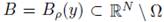
We will say that a domain Ω has a convex-starlike boundary if
 with
with
 for some convex domain Ω1 ⊂
 N, and n(x) · (x - y) < 0 for some y ∈
N and for all x ∈ Γ2. Here n(x) denotes the outward normal to the boundary
, see fig. 2 (a).
N, and n(x) · (x - y) < 0 for some y ∈
N and for all x ∈ Γ2. Here n(x) denotes the outward normal to the boundary
, see fig. 2 (a).
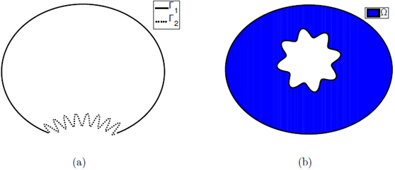
A particular case appears when Q = Qi \ Q 2 with Q 2 c Qi, where Qi is convex, and Q 2 star-like, that is n2(x) • (x - y) > 0, for some y G RN, and for all x G dQ 2 . Here n2(x) denotes the outward normal to the boundary dQ 2 . In that case, we will say that Q is a ring-like domain, see fig. 2 (b). Since (1) is invariant under translations, without loss of generality, we may assume y = 0; in other words, we may assume Q2 to be star-like with respect to zero.
Theorem 1.2. Assume that Ω ⊂
 N
is a bounded C
2
domain with convex-starlike boundary. Let us consider the BVP
N
is a bounded C
2
domain with convex-starlike boundary. Let us consider the BVP
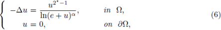
with α > 2/(N - 2).
Then, there exists a uniform constant C, depending only on Ω and f, such that for every classical solution u > 0 to (6),
Proof. It is a Corollary of Theorem 3.1 (see also [8, Theorem 2]). For this particular type of nonlinearities, this result is included in Theorem 1.1. But in the abstrac setting, Theorem 3.1 is not included in Theorem 2.1, because we do not assume f (s)/s 2*-1 to be nonincreasing.
For the proof of Theorem 3.1, we first prove a priori bounds near the convex part of the boundary going back to [11]. Using that the boundary term in the Pohozaev identity on the boundary of a star-like region does not change sign, the proof is concluded.
This paper is organized in the following way. In Section 2 we state and prove our abstract main theorem on a priori bounds for semilinear elliptic equations. In Section 3 we state and prove one abstract theorem on a priori bounds in a class of non convex domains.
We also collect some results on the a priori bounds in a neighborhood of the boundary in two Appendices. In Appendix A we describe the moving planes method, and its consequences when applied to a solution in a convex domain (see Theorem A.8). In Appendix B we apply the moving plane methods on the Kelvin transform, and its consequences for the general case (see Theorem A.12). All those results are essentially well known (see [11]). We include them for the sake of completeness and in order to make precise statements clarifying which hypothesis are needed in the convex case and in the non-convex case.
2. A priori bounds for semilinear elliptic equations
We provide a-priori L∞(Ω) bounds for a classical positive solutions to the boundary value problem (1), where Ω ⊂
 N, N > 2, is a bounded C2 domain, and f is a subcritical nonlinearity.
Our main result in this Section are the following two theorems. The first one is on general smooth domains. The proof can be read in [5], we include it by the sake of completeness.
Theorem 2.1. Assume that Ω ⊂
N
is a bounded domain with C
2
boundary. Assume that the nonlinearity f is locally Lipschitzian and satisfies the following conditions:
(H1)
 is nonincreasing for any s > 0.
(H2) There exists a constant C1 > 0 such that
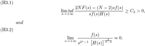
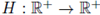
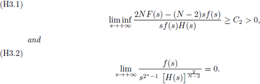
(H3) There exists a constant C2 > 0 and a non-increasing function
 such that
(H4)
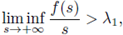 where λ1
is the first eigenvalue of -Δ acting on
where λ1
is the first eigenvalue of -Δ acting on

Then, there exists a uniform constant C, depending only on Ω and f, such that for every classical solution u > 0 to (1),

If the domain Ω is convex, we have the following result:
Theorem 2.2. Assume that Ω ⊂
N
is a bounded, convex domain with C
2
boundary. Assume that the nonlinearity f is locally Lipschitzian, satisfies (H2)-(H4), and also the following conditions:
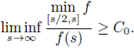
(H1)' There exists a constant C
0
> 0 such that
Then, there exists a uniform constant C, depending only on Ω and f, such that for every classical solution u > 0 to (1),

Our analysis extends previous results, widen the known ranges of subcritical nonlinearities for which positive solutions are apriori bounded and also applies to non-convex domains.
All those results are known (see [5]). We include the proofs for the sake of completeness. Our proofs of Theorem 2.1 and Theorem 2.2, as in [11], use moving plane arguments, the Kelvin transform, and a Pohozaev identity (see [25]). These ideas are well known but we combine them in a slightly different way.
The moving planes method was used by Serrin in [26]. Gidas, Ni and Nirenberg in [14], using this moving planes method and the Hopf Lemma, prove symmetry of positive solutions of elliptic equations vanishing on the boundary. See also Castro-Shivaji [9], where symmetry of nonnegative solutions is established for f (0) < 0. In [14] the authors also characterized regions inside Ω, next to the convex part of the boundary, where a positive solution cannot have critical points. Those regions, called maximal caps, depend only on the local convexity of Ω, and are independent of f and u (see the Appendix A.2 for a precise definition of maximal cap). This non-existence of critical points in a maximal cap, is due to the strict monotonicity of any positive solution in the normal direction. This is a key point to reach local a priori bounds in a neighborhood of the boundary.
The arguments split into two ways, depending on the convexity of the domain. The reason is the following one. If Ω is convex, and the nonlinearity f satisfies (H4), then any positive solution is a priori bounded in a neighborhood of the boundary; more precisely, there exists a constant C depending only on Ω and f but not on u, such that (5) holds (see [11] and Theorem A.8).
If Ω is a general bounded domain, not necessarily convex, the argument on the a priori bounds in a neighborhood of the boundary relies on the Kelvin transform. In that case, if the nonlinearity f satisfies (H1) and (H4), then any positive solution is a priori bounded in a neighborhood of the boundary, in other words, conclusion (5) is reached, (see [11] and Theorem A.12). We include this Theorems in Appendix A and B in order to clarify which hypothesis are needed in the convex case and in the non-convex case respectively. The starting point in the proof of Theorems 2.1 and 2.2 are a priori bounds in a neighborhood of the boundary (Theorems A.12 and A.8, respectively).
In [6] and [7] we study the associated bifurcation problem for a nonlinearity λu+g(u) with g subcritical. We provide sufficient conditions guarantying that either for any λ < λ1 there exists at least a positive solution, or for any continuum (λ,u λ ) of positive solution, there exists a λ* < 0 such that λ* < λ < λ1 and

(see [7, Theorem 2]). In case Q is convex, for any λ < λ1 there exists at least a positive solution (see [6, Theorem 1.2]).
2.3. Proof of Theorems 2.1 and 2.2
Let us start this Subsection with the following remark.
Remark 2.3. By hypothesis,
 is a non-increasing function, therefore 0 ≤ lim s→∞ H(s) < ∞.
By hypothesis (H3.2) we also conclude that
Next, we prove Theorem 2.2 (we recall the ideas collected on Subsection 1.1).
Proof of Theorem 2.2. Step 1. From (5) and de Giorgi-Nash type Theorems (see [20, Theorem 14.1]),

where

From Schauder interior estimates (see [17, Theorem 6.2]),
Finally, combining L p estimates with Schauder boundary estimates (see [3], [17]),

Consequently, there exists two constants C, δ > 0 independent of u such that

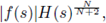
Step 2. From hypothesis (H3.1), there exists a constant C3 > 0 and a non-increasing function H such that

Applying this inequality to any positive solution, and integrating on Ω, we obtain that

for some constant C4 independent of u. From now on, throughout this proof C denotes several constants independent of u.
From a slight modification of Pohozaev identity (see [11, Lemma 1.1] and [25]), if y ∈
 N is a fixed vector, then any positive solution u of (1) satisfies

This, (8) and (7) yield
for some constant C independent of u. Next we prove that also

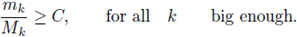
From hypothesis (H4), there exists a constant C such that if s > C then f (s) > 0. Therefore, splitting the above integral in the set S = {x ∈ Ω : |u| ≤ C} and its complementary Ω \ S, since from (9)
 then (10) holds.
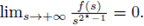
Step 3. From hypothesis (H3.2),
 Multiplying numerator and denominator by
 we can assert that there exists a constant C such that

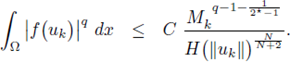
Applying this inequality to any positive solution, integrating on Ω, and using (10) we obtain that
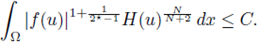
Consequently, since H is non-increasing,
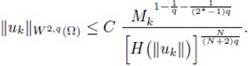
for any q > N/2.
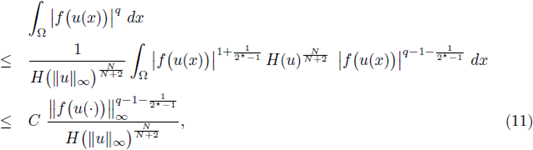
Therefore, from elliptic regularity (see [17, Lemma 9.17]),
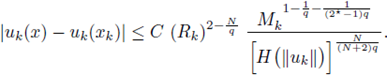
Let us restrict q ∈ (N/2, N). From Sobolev embeddings, for 1/q* = 1/q - 1/N with q* > N we can write
From Morrey's Theorem (see [3, Theorem 9.12 and Corollary 9.14]), there exists a constant C only dependent on Ω, q and N such that

Therefore, for all x ∈ B(x1, R) ⊂ Ω,

Step 4. From now on, we shall argue by contradiction. Let {uk}k be a sequence of classical positive solutions to (1) and assume that

Let C, δ > 0 be as in (5). Let
 be such that
By taking a subsequence if needed, we may assume that there exists
 such
such

Let us choose Rk such that B k = B(xk, Rk) ⊂ Ω, and
and there exists
 such that

Let us denote by

Therefore, we obtain

Then, reasoning as in (11), we obtain
From elliptic regularity (see (12)) we deduce
Step 5. From Morrey's Theorem (see (13)), for any x ∈ B(xk, Rk)
Particularizing x = yk in the above inequality and from (14) we obtain
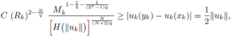
which implies
or equivalently
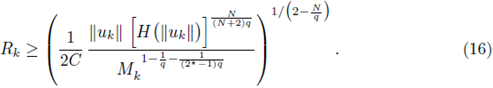
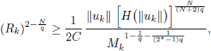
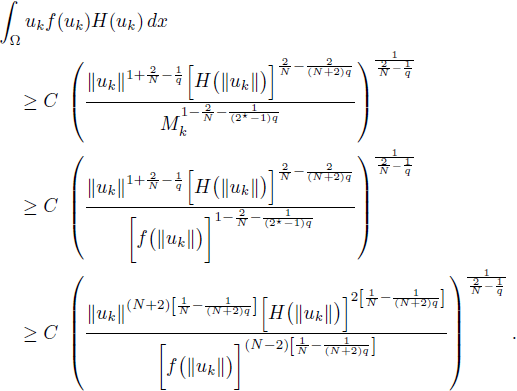
Step 6. Consequently, taking into account (15), and that H is non-increasing,
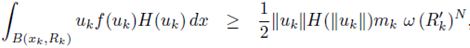
where w = wN is the volume of the unit ball in
 N.
N.
Due to B(xk, Rk) ⊂ Ω , substituting inequality (16), and rearranging terms, we obtain
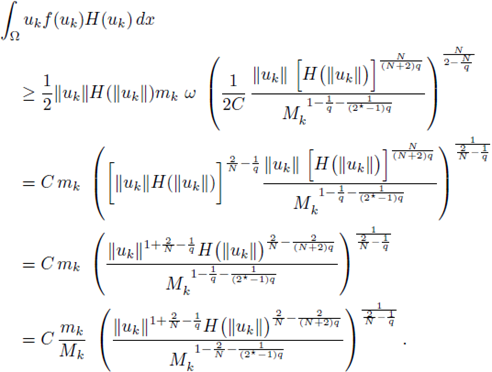
At this moment, let us observe that from hypothesis (H1)' and (H2),
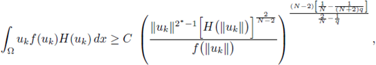
Hence, taking again into account hypothesis (H2), and rearranging exponents, we can assert that
Finally, we deduce
and from hypothesis (H3.2),
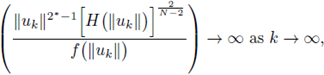
which contradicts (9), ending the proof.
Next, we prove Theorem 2.1:
Proof of Theorem 2.1. Clearly hypotheses (H1) implies hypotheses (H1)'.
For non-convex domains, we use the Kelvin transform to get the a-priori bounds in a neighborhood of the boundary. Let us observe that we need additionally hypothesis (H1) (see Theorem A.12). All the other arguments work exactly in the same way as in the above proof.
3. A priori estimates in a class of non-convex regions
In this Section we prove a priori bounds for the positive solutions to the boundary-value problem

where
 is a bounded C2 domains with convex-starlike boundary, including ring-like regions, and
 is a subcritical nonlinearity.
Let λ1, ϕ
1 stand for the first eigenvalue, first eigenfunction, of the problem - Δϕ
1 = λ1
ϕ
1 in
Our main result is:
Theorem 3.1. Assume that
 is a bounded C
2
domain with convex-starlike boundary. If the nonlinearity f is locally Lipschitzian and satisfies:
is a bounded C
2
domain with convex-starlike boundary. If the nonlinearity f is locally Lipschitzian and satisfies:
(H1) There exist contants C
0
> 0, β
0 ∈ (0,1) such that
(H2) There exists a constant C
1 > 0 such that
(H3) There exists a constant C
2
> 0 and a non-increasing function
 such that
(H4)
 where λ1
is the first eigenvalue of -Δ acting on
where λ1
is the first eigenvalue of -Δ acting on

Then there exists a uniform constant C, depending only on Q and f, such that for every classical solution u > 0 to (17),
Unlike results in [11] or [8], we do not assume
 to be nonincreasing. The proof can be read in [8], we include it here by the sake of completeness.
Proof of Theorem 3.1. Step 1. Due to n(x) · x < 0 for all x ∈ Γ2, we can choose ε > 0 such that if x ∈ Γ1 and d(x, Γ2) < ε, then n(x) · x < 0. Let us
 and
and
From now on, throughout this proof C denotes several constants independent of u. From 5 and de Giorgi-Nash type Theorems (see [20, Theorem 14.1]),

where wt : = {x ∈ Ω : d(x, Γ’ 1 i) < t}.
From Schauder interior estimates (see [17, Theorem 6.2]),
Finally, combining L p estimates with Schauder boundary estimates (see [3], [17]),

Consequently, there exists two constants C, δ > 0 independent of u, such that

Step 2. Any classical solutions to (17) satisfies the following identity, known as Pohozaev identity (see [25]):

where n(x) is the outward normal vector to the boundary at

Since u vanishes on
 , for any tangential vector t(x) we have

Moreover, since
 is a convex-starlike boundary, for each
 we have

and T(x) is tangential to
 . In particular, (20) holds for any x ∈ Γ'2.
Since
 and (20),
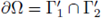
Substituting F(u(x)) = 0 for all
 and (20)-(21) in (19) we have
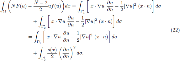
Also, since s(x) ≤ 0 for all x ∈ Γ’2, from (22), and (18),

Next we prove that also

From hypothesis (H4), there exists a constant C such that if s > C, then f (s) > 0. From hypothesis (H3.1), in particular, there exists a constant C such that if s > C, then 2NF(s) - (N - 2)sf (s) > 0. Splitting the above integral in the set S = {x ∈ Ω : |u| ≤ C} and its complement Ω\S, since from (23)
 then (24) holds.
All other arguments work as in Theorems 2.1, 2.2 (see also [8]).
A. Appendix I: The moving planes method, the Kelvin transform, and a priori bounds in a neighborhood of the boundary
In this Appendix, we collect some well-known results on the moving planes method: Theorem A.1 and Theorem A.4. Next, we state results concerning a-priori bounds in a neighborhood of the boundary: Theorems A.8, and A.12. The remaining theorems indicates the arguments through the Kelvin transform, Theorem A.9 fix regions where a Kelvin transform of the solution has no critical points, and Theorems A.10, A.11 translate those results to the solution. All those results are essentially well known (see [11]); we include it here in order to clarify which hypotheses are used in the convex case and in the non-convex case.
A.J. The Kelvin transform
Let us recall that every C2 domain Ω satisfies the following condition, known as the uniform exterior sphere condition:
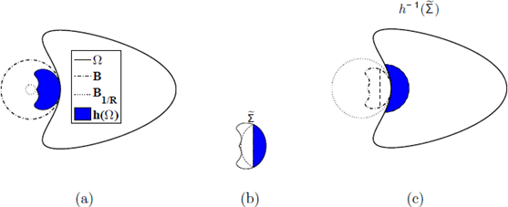
Figure 3 (a) The exterior tangent ball and the inversion of the boundary into the unit ball. (b) A maximal cap
 in the transformed domain h(Ω). (c) The set h
-1
(
) (i.e., the inverse image of the maximal cap
) in the original domain Ω.
in the transformed domain h(Ω). (c) The set h
-1
(
) (i.e., the inverse image of the maximal cap
) in the original domain Ω.
(P) there exists a p > 0 such that for every
 there exists a ball
 such that

Let
 and let
 be the closure of a ball intersecting
 only at the point x0. Let us assume x
0
= (1, 0, … , 0), and B is the unit ball with center at the origin. The inversion mapping
only at the point x0. Let us assume x
0
= (1, 0, … , 0), and B is the unit ball with center at the origin. The inversion mapping

is an homeomorphism from
 into itself; observe that h(h(x)) = x. We perform an inversion from Q into the unit ball B, in terms of the inversion map h|Ω (see fig. 3
(a)).
Let u solve (1). The Kelvin transform of u at the point
 is defined in the transformed domain
 by
by

A.2. The moving planes method
We move planes in the x1-direction to fix ideas. Let us first define some concepts and notations.
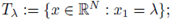

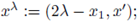
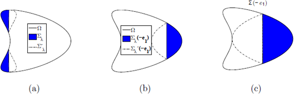
Figure 4 (a) A cap Σλ and its reflected cap
 in the ei direction. (b) A cap Σλ (-e1) and its reflected cap
(-e1) (in the -e1 direction). (c) A maximal cap Σ (-e1).
in the ei direction. (b) A cap Σλ (-e1) and its reflected cap
(-e1) (in the -e1 direction). (c) A maximal cap Σ (-e1).
- the reflected cap:
: = {xλ: x ∈ Σλ (see fig. 4(a));- the minimum value for λ or starting value:
- the maximum value for
- the maximal cap:
.
The following Theorem is Theorem 2.1 in [14].
Theorem A.1. Assume that f is locally Lipschitz, that Ω is bounded and that
 and Σ are as above. If
 satisfies (1) and u > 0 in Ω, then for any λ ∈ (λ0, λ*)

Furthermore, if
 at some point in Ω ∩ Tλ*
, then u is symmetric with respect to the the plane Tλ*
, and
at some point in Ω ∩ Tλ*
, then u is symmetric with respect to the the plane Tλ*
, and
Proof. See [14, Theorem 2.1 and Remark 1, p.219] for f ∈ C 1 and locally Lipschitzian respectively.
Remark A.2. Set
 (see fig. 4(a)). Let us observe that by definition of A0, TAo is the tangent plane to the graph of the boundary at x0, and the inward normal at x0, is ni(x0) = e1. The above Theorem says that the partial derivative following the direction given by the inward normal at the tangency point is strictly positive in the whole maximal cap. Consequently, there are no critical points in the maximal cap.
Now, we apply the above Theorem in any direction. According to the above Theorem, any positive solution of (1) satisfying (H1) has no stationary point in any maximal cap moving planes in any direction. This is the statement of the following Corollary. First, let us fix the notation for a general
 with |v | = 1. We set
- the moving plane defined as:
- the cap: Σλ(V) = {x ∈ Ω : x · v < λ};
- the reflected point: x λ (v) = x + 2(λ - x · v)v;
- the reflected cap:
- the minimum value of
- the maximum value of λ: λ*(z/) = max{λ : Ti' (v) C Ω for all /x < λ};
- and the maximal cap:
Finally, let us also define the optimal cap set
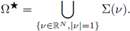
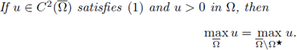
Applying Theorem A.1 in any direction, we can assert that there are not critical points in the union of all the maximal caps following any direction. The set
 is the union of the maximal caps in any direction, and in particular, the maximum of a positive solution is attained in the complement of
. Thus we have:
is the union of the maximal caps in any direction, and in particular, the maximum of a positive solution is attained in the complement of
. Thus we have:
Corollary A.3. Assume that f is locally Lipschitzian, that Ω is bounded, and that
is the optimal cap set defined as above.
If
is a boundary neighborhood of
 in
in
 , as it happens in convex domains, then there is e > 0 depending only on the geometry of Ω (independent of f and u) such that u has no stationary points in a ε-neighborhood of
. Next we study the case in which
is not a neighborhood of
, as it happens in convex domains, then there is e > 0 depending only on the geometry of Ω (independent of f and u) such that u has no stationary points in a ε-neighborhood of
. Next we study the case in which
is not a neighborhood of
 in Ω.
in Ω.
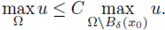
We prove that the maximum of u in the whole domain Ω can be bounded above by a constant multiplied by the maximum of u in some open set strongly contained in Ω (see Theorem A.11 below).
To achieve this result, we will need the moving plane method for a nonlinearity f = f(x, u). Next we study this method on nonlinear equations in a more general setting. Let us consider the nonlinear equation

where
 is a real function, F = F{x, s,p, r) and
 The operator F is assumed to be elliptic, i.e., for positive constants m, M,

On the function F we will assume:
(F1) F is continuous and differentiable with respect to the variables s,p
i
,r
i,j
, for all values of its arguments

(F2) For all
 satisfies either

(F3) F satisfies
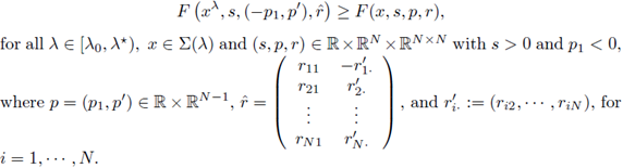
The following theorem is Theorem 2.1' in [14].
Theorem A.4. Assume that Ω is bounded and that
 and Σ are as above. Let F satisfies conditions (F1), (F2) and (F3).
If
 satisfies (27) and u > 0 in Ω, then for any λ ∈ (λ0, λ*)

Furthermore, if
 at some point Ω ∩ Tλ* en necessarily u is symmetric in the plane Tλ*, and

As an immediate corollary in the semilinear situation we have the following one.
Corollary A.5. Suppose
 ¿s a positive solution of

Assume f = f(x, s) and its first derivative f
s
are continuous, for
Assume that

Then for any λ ∈ (λ 0, λ*)

Furthermore, if
 at some point in Ω ∩ Tλ*
, then necessarily u is symmetric in the plane Tλ*, and
at some point in Ω ∩ Tλ*
, then necessarily u is symmetric in the plane Tλ*, and

Set
 The above Theorem says that the partial derivative following the direction given by the inward normal, ni(x0), at the tangency point x0, is strictly positive in the whole maximal cap Σ = Σ (ni(x0)); consequently, the function g(t) := u(x0 + tn¡(x0)) is non-decreasing for t ∈ [0,t0] for some t
0 = t0(x0) > 0.
The above Theorem says that the partial derivative following the direction given by the inward normal, ni(x0), at the tangency point x0, is strictly positive in the whole maximal cap Σ = Σ (ni(x0)); consequently, the function g(t) := u(x0 + tn¡(x0)) is non-decreasing for t ∈ [0,t0] for some t
0 = t0(x0) > 0.
Now consider a neighborhood of x0 denoted by Bδ
0(x0). We can observe that for any
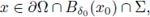 also the function g(t) := u(x + tni(x0)) is non-decreasing for t ∈ [0, t0] for some t0 = t0(x0, x) > 0. By choosing points x such that dist(x, Tλ* (ni(x0))) > δ, we see that the function g(t) := u(x + tni(x0)) is non-decreasing for t ∈ [0, δ] for any
 .
.
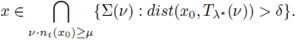
Now, let us move to a different cap, in a neighborhood of x0. We apply the idea, to their corresponding maximal caps Σ, with their corresponding vectors v. Then, choosing points in the intersection of the maximal caps, such that dist(x,Tλ(v)) > δ, also the function g(t) := u(x + tv) is increasing for t ∈ [0, δ]. This is the statement of the following two corollaries, whose ideas are contained in [11].
Corollary A.6. Assume that Ω is bounded and that
 and Σ(v) are as above.
Suppose
 is a positive solution of (28). Assume f = f(x,s) and its first derivative f
s
are continuous, for
is a positive solution of (28). Assume f = f(x,s) and its first derivative f
s
are continuous, for

Let
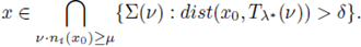
 such that Σ = Σ(ni(x0)) ≠ ∅. Assume also that there exists a μ > 0 such that

where v ∈ ℝN is such that |v| = 1, and v · ni(x0) ≥ μ.
Then, there exists δ > 0 depending only on the geometry of Ω, independent of f and u, such that the following holds:
the function

for any v ∈ ℝN
, such that |v| = 1, v · ni(x0) ≥ μ, and for any
 such that
For each point in a δ /2 neighborhood of the boundary, there exists a cone K depending on the point, such that the function at that point is less or equal than the function at any point of the cone K. Now, we can choose a subset K1 ⊂ K depending on the point, but whose measure can be made independent of the point; remember that the function at that point is still less or equal than the function at any point of the subset K’. This is the statement of the following corollary, whose ideas, as we already said, are included in [11].
Corollary A.7. Assume that Ω is bounded and that
 and Σ(v) are as above. Assume all the hypothesis of Corollary A.6 holds. Let δ > 0 be as described in Corollary A.6.
Then, for any x 1 = x +t 1 v with 0 <t 1 < δ /2, the function

for any v ∈ ℝN
, such that |v| = 1, v · ni(x0) ≥ μ, and for any
 such that
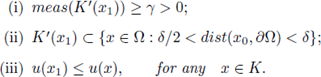
Moreover, there exists a positive number γ (depending only on the geometry of Ω, and independent of f and u), such that:
for any x
1
= x + t1 v with 0 < t1
< δ /2, there exists a cone with vertex
 and a piece of that cone K' = K'(x
1
) such that
and a piece of that cone K' = K'(x
1
) such that
A.3. A priori bounds in a neighborhood of the boundary
From now on, the arguments split into two ways, depending on the convexity of the domain. If Ω is convex, we observe that, reasoning as in [11], specifically, using Corollary A.6 and Corollary A.7, any positive solution u is locally increasing in the maximal cap following directions close to the normal direction, which provides L∞ bounds locally in a neighborhood of the boundary. This is the statement of the following Theorem.
Theorem A.8. Assume that Ω ⊂ ℝN is a bounded, convex domain with C 2 boundary. Assume that the nonlinearity f satisfy (H4).
If
 satisfies (1) and u > 0 in Ω, then there exists a constant δ > 0 depending only on Ω and not on f or u, and a constant C depending only on Ω and f but not on u, such that

Proof. As observed in [4], [11, p. 44], [23], [27], under hypothesis (H4), there exists a constant C 1 > 0 such that

for any u solving (1).
Next, we will use Corollary 3.7. Let us fix an arbitrary
 and let n
i
(x
0
) be the inward normal at the boundary point x
0
. Choose any v ∈ ℝN such that |v | = 1, and v · n
i
(x
n
) ≥ μ for some μ > 0 fixed. From Corollary 3.6, there exists a δ > 0 depending only on the geometry of Ω, and independent of f and u, such that the function g(t) := u(x + tv) is non decreasing for any t ∈ [0,δ], and for any
and let n
i
(x
0
) be the inward normal at the boundary point x
0
. Choose any v ∈ ℝN such that |v | = 1, and v · n
i
(x
n
) ≥ μ for some μ > 0 fixed. From Corollary 3.6, there exists a δ > 0 depending only on the geometry of Ω, and independent of f and u, such that the function g(t) := u(x + tv) is non decreasing for any t ∈ [0,δ], and for any
 in a certain neighborhood of x
0. The neighborhood of x
0 depends only on the convexity of Ω, and it is independent of f and u.
in a certain neighborhood of x
0. The neighborhood of x
0 depends only on the convexity of Ω, and it is independent of f and u.
Taking into account that all the hypotheses of the mentioned Corollary 3.7 hold, and using specifically Corollary 3.7 (iii), we deduce that for any x1 = x+t1 v ∈ Ω, with 0 <t1 < δ/2, there exists a cone with vertex
 and a piece ot that cone
 such that |K'| ≥ γ > 0, and

Taking into account (30), (31), and Corollary 3.7 (i), we deduce that

Consequently, there exists a constant C only dependent on f and on the geometry of Ω such that

Then there exists a constant δ > 0, depending only on Ω and not on f or u, and a constant C depending only on Ω and f but not on u, such that (29) holds. 0
Next, we go through the non-convex case, reasoning on the Kelvin transform. First, in Theorem A.9, we fix regions where a Kelvin transform of the solution has no critical points. This is the statement of the following theorem, whose ideas are contained in [11]. Let us fix some notation. For any
 be the inward normal at x
0 in the transformed domain
be the inward normal at x
0 in the transformed domain
 where h is defined in (25), and let
 be its maximal cap (see fig. 3(b)).
Theorem A.9. Assume that Ω ⊂ ℝN is a bounded domain with C 2 boundary. Assume that the nonlinearity f satisfies (H1).
If u
 satisfies (1) and u > 0 in Ω, then for any
 its maximal cap in the transformed domain
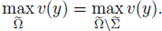
 is nonempty, and its Kelvin transform v, defined by (26), has no critical point in the maximal cap
.
is nonempty, and its Kelvin transform v, defined by (26), has no critical point in the maximal cap
.
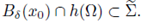
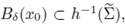
Consequently, for any
, there exists a δ > 0 only dependent of Ω and x
0
, and independent of f and u, such that its Kelvin transform v has no critical point in the set Bδ(x0) ∩ h(Ω).
Proof. Since Ω is a C
2 domain, it satisfies a uniform exterior sphere condition (P). Let
, and let
 be the closure of a ball intersecting
 only at the point x0. For convenience, by scaling, translating and rotating the axes, we may assume that x0
= (1 , 0, … , 0), and B is the unit ball with center at the origin.
only at the point x0. For convenience, by scaling, translating and rotating the axes, we may assume that x0
= (1 , 0, … , 0), and B is the unit ball with center at the origin.
We perform an inversion h from Ω into the unit ball B, by using the inversion map
 Due to
 and to the boundedness of Ω, there exists some R> 0 such that

and the image

Note that
 (see fig. 3(a)). Moreover, Ω is strictly convex near x0 and the maximal cap
 contains a full neighborhood of x0 in
 where ñi(x0) is the normal inward at x0 (see lemma B.1 in the Appendix; see also fig. 3(b)). Observe that, by construction ñi(x0) = -e
1
.
where ñi(x0) is the normal inward at x0 (see lemma B.1 in the Appendix; see also fig. 3(b)). Observe that, by construction ñi(x0) = -e
1
.
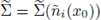
Next, we consider the Kelvin transform of the solution defined by (26). The function v is well defined on h(Ω), and writing
 and Δw for the Laplace-Beltrami operator on
 the function v satisfies
Therefore, v > 0 in
 satisfies

From hypothesis (H1), we see that the function

satisfies the hypothesis of Corollary A.5. By construction, it is straightforward that |yλ| < |y| for all y ∈
(see fig. 3 (a) and (b), and remain that the origin is at the center of the ball B). By (H1),
where
is the maximal cap in the transformed domain (see fig. 3 (b)). Therefore, the hypotheses of Corollary A.5 are fulfilled, and hence v has no critical point in the maximal cap
, which completes the proof choosing δ such that
We are now ready to state the following theorem, essentially contained in [11]. This result is composed of two theorems: the first one, Theorem A.10 below, is the local version in a neighborhood of a boundary point; the second one, Theorem A.11, is the global version.
Theorem A.10. Assume that Ω ⊂ ℝN is a bounded domain with C 2 boundary. Assume that the nonlinearity f satisfies (H1).
If u
 satisfies (1) and u > 0 in Ω, then for any
 there exists a δ > 0 only dependent of Ω and x
0
, and independent of f and u such that
there exists a δ > 0 only dependent of Ω and x
0
, and independent of f and u such that
The constant C depends on Ω but not on x 0 , f or u.
Proof. Let
; if there exists a δ > 0 such that
 (as it happens in convex sets), the proof follows from Theorem A.9. We concentrate our attention in the complementary set.
Let
 , and let
 be the closure of a ball intersecting
 only at the point x0
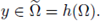
. Let v be as defined in (26) for
only at the point x0
. Let v be as defined in (26) for
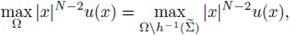
 By a direct application of Theorem A.9, v has no critical point in the maximal cap Σ, and therefore
From definition of v, see (26), we obtain that
where
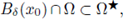
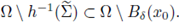
 is the inverse image of the maximal cap (see fig 3(b)-(c)). Due to the boundedness of Ω (see (32)), we deduce
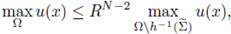
which concludes the proof choosing C = RN-2 and δ such that
 and therefore
The following Theorem is just a compactification process of the above result.
Theorem A.11. Assume that Ω ⊂ ℝN is a bounded domain with C 2 boundary. Assume that the nonlinearity f satisfies (H1).
If
 satisfies (1) and u > 0 in Ω, then there exists two constants C and δ depending only on Ω and not on f or u such that
where

Proof. Since Ω is a C2 domain, it satisfies a uniform exterior sphere condition (P). Thanks to that property, we can choose a constant C = (R/p) N-2 satisfying the above inequality.
Moreover, let us note that from Theorems A.9 and A.10, the constant S only depends on geometric properties of the domain Ω.
Finally, we observe that, reasoning as in [11] on the Kelvin transform, specifically using Corollary A.6 and Corollary A.7, the Kelvin transform of u at
 is locally increasing in the maximal cap of the transformed domain, which provides L∞ bounds for the Kelvin transform locally. By a compactification process, we then translate this into L°° bounds in a neighborhood of the boundary for any solution of the elliptic equation. This is the statement of the following theorem.
Theorem A.12. Assume that Ω C RN is a bounded domain with C 2 boundary. Assume that the nonlinearity f satisfies (H1) and (H4).
If
 satisfies (1) and u > 0 in Ω, then there exists a constant δ > 0 depending only on Ω and not on f or u, and a constants C depending only on Ω and f but not on u, such that

where

Proof. We shall reason as in the proof of Theorem A.8. As observed in [4], [11, p. 44], [23], [27], under hypothesis (H4), there exists a constant C1 > 0 such that

for any u solving (1).
Let us fix an arbitrary
 and consider the Kelvin transform of u at the point
 , denoted by v = v(x0).
Next, we use Corollary A.7 on the Kelvin transform. We only need to note that, by construction, it is straightforward that there exists a
 such that for any v ∈ ℝN such that |v| = 1 and
 (observe that ñi(x0) = ne(x0)), the following holds:

(see fig. 3 (a) and (b), and remember that the origin is at the center of the ball E); then, by (H1), and taking into account the definition of g (see (33)), we obtain

Therefore, all the hypothesis of Corollary A.7 hold. Now, using Corollary A.7 (iii), we deduce that there exist
 only dependents on the geometry of Ω, such that for any
 with
with
 there exists a cone
 and a subset
 such that
 and
and

From definition of v, there exists a constant C only dependent on the geometry of Ω such that

where x1 = h-1(y1), x = h-1(y).
Taking into account (35), (36), and Corollary A.7 (i), we deduce that

Consequently, there exists a constant C only dependent on f and on the geometry of Ω such that

Now we move
 and consider their corresponding Kelvin transforms. By a compactification process, there exists a constant δ > 0 depending only on Ω and not on f or u, and a constants C depending only on Ω and f but not on u, such that (34) holds.
B. On the maximal cap in the transformed domain through the inversion map
In this Appendix we show that for any boundary point of a C2 domain, the maximal cap in the transformed domain is nonempty. This is a known result, but we include it here by the shake of completeness.
This result could see m surprising in presence of highly oscillatory boundaries. For example, assume that the boundary of Ω includes
 (to visualize the scale, see in fig.

Let h(Γ2) be the image through the inversion map into the unit ball B, and let Γ3 be the arc of the boundary
 given by
 (see fig. 5(c)). At this scale, the oscillations are not appreciable. We plot in 5(d) the derivative of the "vertical" distance between the boundary Γ2 and the ball, concretely we plot f'(x) - g'(x) for x ∈ [-0.01,0.01]. We plot in 5(e) the second derivative of the "vertical" distance between the boundary and the ball, which is f ''(x) - g''(x) for x ∈ [-5 · 10-4, 5 · 10-4]. Let us observe that this second derivative is strictly positive, and that f ''(0) - g''(0) = 1. Consequently, the first derivative is strictly increasing, and therefore the "vertical" distance f(x) - g(x) does not oscillate.
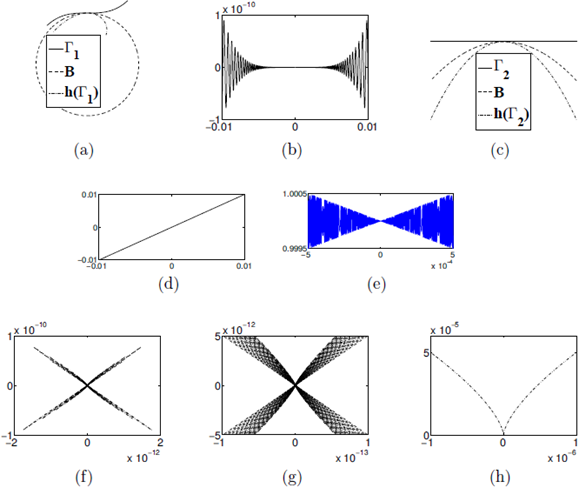
Figure 5 (a) An inflection point at the boundary Γ1 joint with the inversion h(Γ), and the unit circumference; (b) A degenerated critical point at the boundary Γ2; (c) Γ2 joint with its inversion into the unit ball, h(Γ2 ), and the arc of circumference, Γ3 ; (d) f ' (x) - g'(x) for x ∈ [-0.01, 0.01]; (e) f''(x) - g''(x) for x ∈ [-5 · 10-4, 5 · 10-4]; (f) Second coordinate of the difference h(Γ2 ) - h(x, 1), where h(x, 1) is the image of the straight line y =1; (g) a zoom of the same graphic; (h) Second coordinate of the difference h(Γ2) - h(Γ3).
Moreover, let us consider the image through the inversion map of the straight line y = 1, i.e. h(x, 1) = h ({(x, 1), x ∈ [-0.01, 0.01]}). In fig. 5(f)-(g) we plot the second coordinate of the difference h(Γ2) - h(x, 1). The oscillation phenomena is present here. In fig. 5(h) we plot the second coordinate of the difference h(Γ2) - h(
). This difference does not oscillate.
In fig. 5(a) we draw the inversion of the boundary into the unit ball at an inflexion point; more precisely we set
 which has an inflexion point at x = 0.
Let h denote the inversion map defined in (25), and let
 denote the image through the inversion map into the ball B. For any
 ) be the normal inward at x0 in the transformed domain
 and let
 ) be its maximal cap (see fig. 3(b)).
Lemma B.1. If Ω ⊂ ℝN
is a bounded domain with C2
boundary, then for any
 , there exists a maximal cap
 non empty.
Proof. For convenience, we assume x0 = (0, … , 0, 1), and B is the unit ball with center at the origin such that
 denote a parametrization of
 in a neighborhood of x0. Hence,

Let h(Ω) stand for the image through the inversion map into the unit ball. From definition,
 is given by
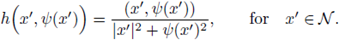
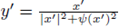
Set y = h(x', ψ(x')) for
 and with y = (y', yN). Since

for
 , then
 for
for
 where
where
 if, and only if,
 for some
 . Therefore,
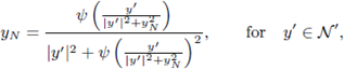
and

where

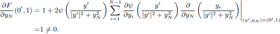
Differentiating (38) with respect to yN we obtain
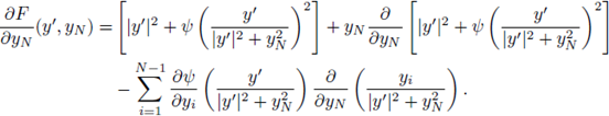
Substituting at (y , yN) = (0 , 1) and taking into account (37),
Therefore, by the Implicit Function Theorem there exists an open neighborhood of 0 , Bδ(0') ⊂ ℝN-1, and a unique function
 such that ϕ(0') = 1, and

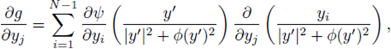
Differentiating (39) with respect to yj, j = 1, … , N - 1, using the chain rule and substituting at the point (0 , 1), we obtain

On the other hand, differentiating (38) with respect to y¿ and using the chain rule we obtain
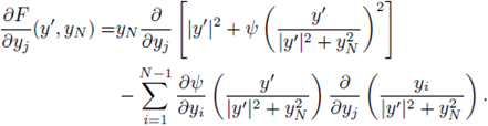
Substituting at (y',y N) = (0', 1) and taking into account (37),
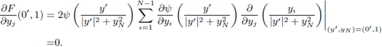
Consequently, by (40)

Let us define

By (37), g(0') = 1, and G(0') = 1. Moreover,

And

Let us see that there exists 0 < δ' ≤ δ such that

is a convex set. To achieve this, we use a characterization of convexity in the twice continuously differentiable case (see [13, p. 87-88]). The set U is a convex set if, and only if, D 2 G(y') is negative semidefinite for all y' ∈ B δ (0'). In fact, we will prove that D 2 G(0') is negative definite and by continuity, there exists some δ' > 0 such that D 2 G(y') is negative semidefinite for all y' ∈ Bδ' (0'). Differentiating,
And

where
 Substituting at y' = 0', and taking into account (37), we deduce

Taking second derivatives for k = 1, … N - 1, we obtain
And
where
 Substituting at y' = 0', and taking into account (37), we deduce
Substituting at y’ = 0’ , and taking into account (42), we deduce
Due to
where δ ij is the Kronecker's delta, substituting at y ' = 0 ', and taking into account (41), we can write
Moreover,

substituting at y’ = 0’ , and taking into account (43), we can write
Let then,

where IN-1 is the identity matrix.
From hypothesis
 Therefore the 'vertical' distance (distance in the x
N coordinate) between
Therefore the 'vertical' distance (distance in the x
N coordinate) between
 and
and
 is strictly positive, i.e.,

or equivalently

Set
 for
for
 with
with
 Then H(0') = 1, and from the above inequality the point x' = 0' is an strict minimum of the function H. Due to (37) every derivative of H evaluated at 0' is zero, and necessarily the Hessian matrix of H must be semi-positive definite, i.e.,
is a semi-positive definite matrix. Hence the matrix -(A + 2I
N-1
) is negative definite, and y' = 0' is a strict maximum of the function G. As a consequence, there exists a δ’ > 0 such that the matrix
 is negative definite for all y’ ∈ Bδ’ (0’). Consequently, the set U is a convex set.
Le us now choose
 Due to y' = 0' is a strict maximum of the function G, and that G(0') = 1, then γ < 1. The cap
 and its reflection
 are non empty sets contained in h(Ω). Hence the maximal cap
 contains
 which is nonempty, and concludes that the maximal cap
is a nonempty set.
which is nonempty, and concludes that the maximal cap
is a nonempty set.


