


 Inglés (pdf)
 Articulo en XML
 Referencias del artículo
 Enviar articulo por email
 Citado por SciELO
  Citado por Google
  Similares en
SciELO
Similares en
SciELO  Similares en Google
 Permalink


1. Introduction
In this part II, we describe our a priori bounds results on semilinear elliptic systems, on quasilinear elliptic equations for the p-laplacian, and the asymptotic behavior of radial solutions as α → 0+ in several subsections. We leave the proofs for the following sections.
In a previous paper containing part I, when p = 2, we show the existence of L∞ a-priori bounds for classical, positive solutions of semilinear elliptic equations Δu = f(u) with Dirichlet homogeneous boundary conditions, for
Appealing to the Kelvin transform, we extend our results to non-convex domains (see [16], [17]).
1.1. Hamiltonian elliptic systems
We provide a-priori L∞(Q)-bounds for classical positive solutions of Hamiltonian elliptic systems
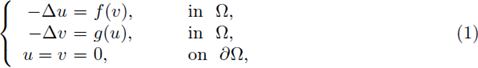
where Ω ⊂ ℝN, N ≥ 2, is a bounded, convex C3 domain,

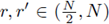
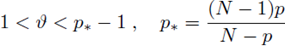
and p, q, are in the so called critical Sobolev hyperbola

(see [71] and Theorem 1.1).
Using these a priori bounds, and local and global bifurcation techniques, we prove the existence of positive solutions for a corresponding parametrized semilinear elliptic system (see [71] and Theorem 1.3).
If the exponents α = β = 0, then we have the Lane-Emden system
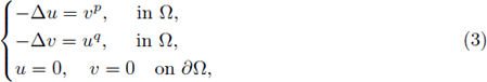
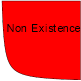
where Ω ⊂ ℝN is either a bounded, smooth subset, or a half space, or ℝN. The exponents (p, q) play a crucial role for the existence or nonexistence of positive solutions of Lane-Emdem system, depending on the boundedness or not of Ω. When Ω is a bounded smooth star-shaped domain, the Sobolev hyperbola divides, on the pq-plane, existence and nonexistence of positive solutions of the Lane-Emdem system (see fig. 1; we include the details in Section 2). When Ω = ℝN there is a conjecture: the hyperbola (2) is also the dividing curve between existence and nonexistence for the Lane-Emdem system.
We now state our main results on elliptic systems. See Section 2, or [71, Theorems 1.1, 1.3] for a proof.
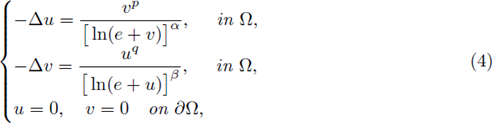
Theorem 1.1 (a-priori L∞ bounds). Let us consider the following semilinear elliptic system:
where Ω ⊂ ℝN
, N ≥ 3, is a bounded, convex domain with boundary
 of class C
2
.
of class C
2
.
Suppose that
 p, q are on the critical Sobolev hyperbola (2), and assume that

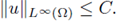
Then there exists a uniform constant C, depending only on Ω and p, q, α, β but not on (u, v), such that

for all positive solutions (u,v) of (4).
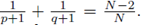
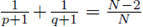
Remark 1.2. Observe that condition (2) relates the exponents p and q to the Sobolev hyperbola, and condition (5) ensures that our nonlinearities are nondecreasing since it will be needed in the proof. Notice that
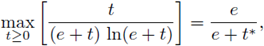
where t* is the solution of the logarithmic equation e ln(e + t) = t.
In the next theorem, we state the existence of positive solutions for the semilinear bipa-rameter elliptic systems (4).
Theorem 1.3 (Existence). Consider the biparameter elliptic system
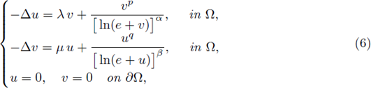
where the exponents p, q, α, β are as defined in Theorem 1.1, and the parameters λ and μ are non-negative real parameters.
Then (6) has a positive solution (u,v) if, and only if,
 where λ1
is the principal eigenvalue associated with the linear eigenvalue problem with homogeneous Dirichlet boundary conditions -Δϕ = λϕ in Ω; ϕ = 0 on
where λ1
is the principal eigenvalue associated with the linear eigenvalue problem with homogeneous Dirichlet boundary conditions -Δϕ = λϕ in Ω; ϕ = 0 on

Proof. See Section 2, or [71, Theorem 1.3] for a proof. 0
The ideas of the proof of Theorem 1.1 are adapted for systems. Moving planes for system provides L∞ bounds in a neighborhood of the boundary of a convex domain, for classical positive solutions of (1). Rellich-Pohazev identity for systems give us two bounded integrals in Ω. With the help of Morrey's Theorem, we estimate the radius R, (R 1 ), of a ball where the function u, (v), exceeds half of its L∞ bound. Then, we get a lower bound of the above integrals, deriving the L∞ bounds for classical positive solutions of (4).
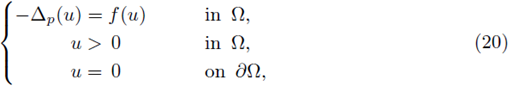
1.2. The p-Laplacian
We consider the Dirichlet problem for positive solutions of the equation - Δp(u) = f (u) in a convex, bounded, smooth domain Ω ⊂ ℝN, with f locally Lipschitz continuous. We provide sufficient conditions guarantying L∞ a priori bounds for positive solutions of some elliptic equations involving the p-Laplacian and extend the class of known nonlin-earities for which the solutions are L∞ a priori bounded. As a consequence we prove the existence of positive solutions in convex bounded domains.
Specifically, in case of elliptic equations involving the p-Laplacian, we prove the existence of a-priori bounds for
 positive solutions of elliptic equations

When

see Example 1 in [31].
Corollary 1.4. Assume that Ω ⊂ ℝN
is a smooth bounded convex domain, 1 < p < N, and u > 0 is a
 solution to
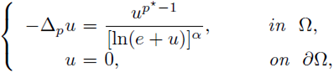
with α > p/(N - p).
Then, there exists a uniform constant C, depending only on i and f but not on the solution, such that
Proof. It is a Corollary of Theorem 3.5 (see also [31, Theorem 1.7 and Example 1 in p. 491]).
1.3. Final remarks
We finally provide sufficient conditions for a uniform L2 (Ω) bound to imply a uniform L ∞ (Ω) bound, for positive classical solutions to a class of subcritical elliptic problems in bounded C 2 domains. We also establish an equivalent result for sequences of boundary value problems.
We also study the asymptotic behavior of radially symmetric solutions u α = u α (r) to the subcritical semilinear elliptic problem
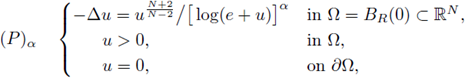
as a → 0+. We prove that there exists an explicitly defined constant L(N, R) > 0, only depending on N and R, such that
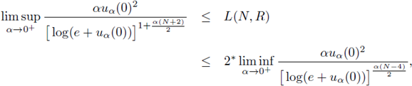
see [75].
This paper is organized in the following way. Section 2 is devoted to semilinear elliptic systems. In Section 3 we state an abstract theorem on a priori bounds for p-laplacian equations in convex domains. Section 4 contains a result on the equivalence between uniform L2* (Ω) a-priori bounds and uniform L∞ (Ω) a-priori bounds for subcritical elliptic equations. In Section 5 we study the asymptotic behavior of radially symmetric solutions u α = u α (r) as α → 0+. In Section 6 we collect some open problems.
2. A priori bounds and existence of positive solutions for semilinear elliptic systems
It is natural to ask whether it is possible to obtain the corresponding a priori results for systems. In this Section, we extend the results of [16] from scalar equations to systems. The existence of a-priori bounds for the system (4) is proved in the same lines of [16], that is, using the Rellich-Pohozaev identity and the method of moving planes as in [21], combined with Morrey's Theorem. The moving planes method is used to obtain L∞ bounds in a neighborhood of the boundary for classical positive solutions of (4), whereas the Rellich-Pohozaev identity is used to get two bounded integrals in i. Furthermore, Morrey's Theorem is used to estimate the radius R, (R'), of a ball where the function u, (v), exceeds half of its L∞ bound (see fig. 2), allowing us to reach a contradiction on the lower bounds of the above integrals.
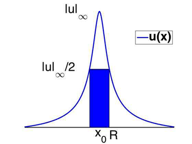
Figure 2 Let (u, v) be a solution of (1); we plot one component u, its L∞ norm, and the estimate of the radius R such that
 for all
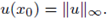
 where x0 is such that
We consider the semilinear elliptic system given by (4) where Ω ⊂ ℝ
N, N ≥ 3, is a bounded, convex domain with a smooth boundary  (at least of class C3), and 1 < p,q < ∞, α, β > 0. The purpose of this Section is to establish a-priori estimates for positive classical solutions of (4) and subsequently prove an existence result for the parametrized version for the system. By a positive classical solution of (4), we mean (u, v) that satisfies (4) and both components are positive. Let us mention that when the exponents α = β = 0, we have the system
that is usually referred to as the Lane-Emden system. This problem arises in modeling spatial phenomena in a variety of biological and chemical problems. Naturally positive solutions of system (7) is of particular interest, and there have been significant studies of positive solutions of (7) where Ω is either a bounded, smooth subset of ℝN, a half space, or the entire space ℝN (see [11], [12], [14], [21], [23], [40], [39], [72], [76], [79], [86], [87], [92] and references therein).
It is known that the pair of exponents (p, q) plays a crucial role in the questions of existence and nonexistence of positive solutions of (7). For instance, it has been shown that on a bounded smooth star-shaped domain Ω ⊂ ℝN, the Sobolev hyperbola (2) is precisely the dividing curve on the pq-plane between existence and nonexistence of positive solutions of (7) (see [21], [72], [76]).
In [21], the authors established a-priori estimates and proved the existence of positive solutions of (7) when (p, q) is subcritical (i.e. (p, q) lies below the critical Sobolev hyperbola), that is,
 Moreover, in [72], the author proved that if (p, q) is critical (i.e. (p, q) lies on critical Sobolev hyperbola) or supercritical (i.e. (p, q) lies above the critical Sobolev hyperbola), namely if
 then (7) has no positive solution (see fig. 1).
When Ω = ℝN, it has been conjectured that the hyperbola (2) is also the dividing curve between existence and nonexistence for (7). The conjecture has been completely proved for radial positive solutions (see e.g. [72], [85]), that is, if (p, q) is subcritical, then there are no radial positive classical solution to (7) (see [72] for p > 1, q > 1) and it has been extended in [85] for the case p > 0 and q > 0. Furthermore, if (p, q) is critical or supercritical, system (7) does admit (bounded) positive radial solutions (see e.g. [72], [85]). In the more general case, i.e. without assuming radial symmetry, the question has not been completely answered yet. Partial answers are known for nonexistence of positive entire solutions of (7) when the pair of exponents are subcritical; for example, it has been proved the nonexistence in certain space dimensions [72], [87] or in certain subregions, below the critical hyperbola in the (p,q)-plane (see e.g. [14], [87]). For
 (i.e. the half space), we refer to [11] for the study of nonexistence of positive solutions. These nonexistence results in ℝN or ℝN allow to prove a-priori bounds for positive solutions of semilinear elliptic equations in bounded domains via the blow-up method (see e.g. [52], [53], [11], [92]).
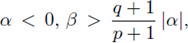
In the present Section, we use the method of moving planes and the Rellich-Pohazev identity for systems to establish a-priori L∞ bounds when the pair of exponents (p, q) lies on the critical Sobolev hyperbola (2) and
 and then subsequently prove an existence result for the parametrized version for the system (see system (6) below). Problems of type (4) has been considered by several authors (we refer to [37], [22]). In [37, Theorem 1.3] the authors study the existence of solutions of (4) when the pair of exponents (p,q) lies on the critical Sobolev hyperbola (2) and
 that is, one nonlinearity is above the power function. Whereas in [22, Theorem 2.7] the authors study related nonlinearities when the pair of exponents (p, q) lies below the critical Sobolev hyperbola (2), using variational approaches.
Throughout this Section we assume that Ω ⊂ ℝN is a smooth bounded, convex domain. The hypothesis on convexity of the domain is needed in order to establish a priori bounds in a neighborhood of the boundary, via the moving planes method (see Lemma 2.1). In [89, Lemma 4.3] the author develop the moving planes method for systems assuming that both nonlinearities are nondecreasing and do not depend explicitly on the spatial variable x.
Let us first briefly recall the different methods for deriving a-priori estimates for elliptic systems in the literature. In [93], the existence of a-priori estimates of classical positive solutions of (4) was proved based on scaling or blow-up method which requires the nonlinearities to have a precise asymptotic behavior at infinity, typically f ~ v p , g ~ uq. In [79], [80], the authors derived a-priori estimates results using a method close to the Hardy-Sobolev inequalities method. This method requires only upper bounds on the growth of the nonlinearities and allows the nonlinearities to depend on x, u and v, but the growth bounds assumed on f, g are more restrictive than in general.
For elliptic equations on general bounded domains, not necessarily convex, de Figueiredo, Lions and Nussbaum [40] applied the moving planes method on the Kelvin transform in order to avoid the difficulty of an empty cap (see [51], [16] for details and the definition of a cap). In that situation, it turns out that the (transformed) nonlinearity depends on the spatial variable x. Then, they obtained a priori bounds in a neighborhood of the boundary for classical positive solutions of scalar equations on non-convex domains. To the best of our knowledge, the moving planes method for systems is not yet developed for nonlinearities depending also on the variable x. Hence, we focus on convex domains.
The ideas of the proof of Theorem 1.3 are based on local bifurcation techniques [24], combined with global bifurcation theorem [34], [63], [82], and the a-priori estimates. From the seminal works of Crandall and Rabinowitz (see [24], [82]), there are a huge amount of references corresponding to one-parameter bifurcation theory. There are not so many on multiparameter bifurcation. Let us mention Alexander and Antman's Theorem [3] on global multiparameter bifurcation techniques, looking for a change of fixed point index, and providing a manifold of solutions of topological dimension at least the number of parameters, [64] on local multiparameter bifurcation techniques on elliptic systems, [48], [63], [64], [65], [66], [67], [68] on combination of local and global multiparameter bifurcation techniques on elliptic systems, and [49] on the multiparameter bifurcation for the p-laplacian.
In this Section, we state two lemmas that are relevant in order to obtain the a priori estimates. The first lemma provides L°° a priori bounds for any positive solution of (4) in a neighborhood of the boundary (see [40]). The hypothesis of convexity of the domain is needed in order to establish these a priori bounds in a neighborhood of the boundary. Whereas the second lemma provides a Rellich-Pohozaev-Mitidieri type identity (see [72] for a proof).
Lemma 2.1. Let (u,v) be a positive classical solution of the system (4). Assume that the hypotheses of Theorem 1.1 are satisfied. Then there exists a constant δ > 0 depending only on Ω and not on p, q, α, β or (u,v), and a constant C depending only on Ω and p, q, α, β, but not on (u,v), such that

where

The proof is done in a similar way as step 2 in the proof of Theorem 1.1 in [40], using the moving planes method for systems [89, Lemma 4.3]. See also step 1 and 2 in the proof of Theorem 2.1 in [21].
Lemma 2.2 (Rellich-Pohozaev-Mitidieri type identity). Let u and v be in
 where Ω is a C
1
domain in ℝN
, and u = v = 0 on
where Ω is a C
1
domain in ℝN
, and u = v = 0 on
 . Then,
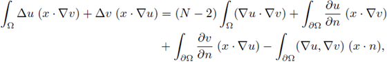
where n denotes the exterior normal, and (x · n) denotes the inner product.
The proof of Theorem 1.1 and Theorem 1.3 can be read in [71]; we include it below by completeness.
Proof of Theorem 1.3. Step 1. It follows from (8) and de Giorgi-Nash type Theorems for systems (see [59, Theorem 3.1, p. 397]) that

where
 Using Schauder interior estimates (see [54, Theorem 6.2]),
Finally, combining L p estimates with Schauder boundary estimates (see [13], [54], [59]),

By the Sobolev embedding for p > N, we have that there exists two constants C, δ > 0, independent of u, such that

Step 2. Let θ ∈ (0,1) be such that

which is possible by (2).
Integrating by parts and taking into account (10) we have that

Likewise

Now, if we set W(s,t) := F(t) + G(s), then W s = g(s) and W t = f (t). Therefore, for solutions u > 0 and v > 0 of (4),
and
Applying Lemma 2.2 (Pohozaev-Rellich-Mitidieri type identity) we get that
Therefore, it follows from (13) and (9) that

Using (11), (12), and (14), we obtain that
Moreover,
and
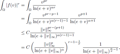
Therefore, for any ε > 0 there exists a constant tε, such that if t >t ε , then
and
Let us choose  then there exists a constant C > 0 such that for any t > 0,
and
Hence, applying the above inequalities for any v(x) and u(x) solving (4) respectively, integrating in Ω and using (15), we have that

This implies that
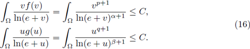
As pointed out in Remark 1.2, condition (5) ensures that f and g are nondecreasing.
Step 3. Now, let us fix
 such that
 and
and
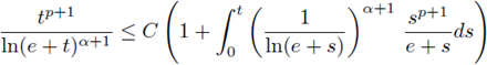
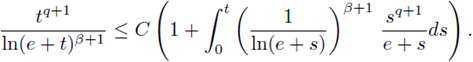
 Then using (16) and the fact that f and g are nondecreasing for
 large enough, we get that
and similarly
All the other arguments work as in part I, Theorems 2.1, 2.2 (see also [71, proof of Theorems 1.1 and 1.3]). 0
Proof of Theorem 1.3. The proof is divided in two parts. We first prove that if there exists a positive solution ((λ, μ), (u, v)) of equation (6) with λ, μ ≥ 0, then
 In the second part, we prove the converse.
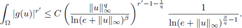
Part I. Assume that there exists a positive solution ((λ, μ), (u, v)) of equation (6), and that λ, μ ≥> 0. Let ϕ1 > 0 be the principal eigenfunction associated to A1 and normalized in the L2(Ω) norm. Multiplying each equation of (6) by ϕ1, and integrating by parts on Ω, it yields that
Multiplying the first equation by λ1, the second equation by λ and adding both equations we deduce
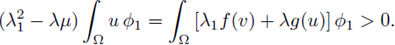
Thus,

Part II. Assume that λ, μ ≥ 0 and
 we will prove that there is a positive solution (u,v) of (6). The proof is divided in three steps. In step 1, we reformulate problem (6) in abstract (operators) setting. In step 2, we fix one parameter, say, λ = λ0
> 0, and choosing μ as bifurcation parameter, we use Crandall-Rabinowitz's Theorem to prove that when
we will prove that there is a positive solution (u,v) of (6). The proof is divided in three steps. In step 1, we reformulate problem (6) in abstract (operators) setting. In step 2, we fix one parameter, say, λ = λ0
> 0, and choosing μ as bifurcation parameter, we use Crandall-Rabinowitz's Theorem to prove that when
 there is a bifurcation phenomena from the trivial solution. Moreover, at least locally, the nontrivial solution pairs (u, v) are strictly positive. In step 3 we use the global bifurcation result stated by Rabinowitz [82] and completed by Dancer [34] (see also [35], [63]) to prove that equation (6) has at least one solution. We conclude with a remark on the fact that varying λ we obtain a whole curve of non-isolated bifurcation points, and using Alexander and Antman's result [3], we can deduce that in a neighborhood of that curve, there is a bifurcating two-dimensional surface of nontrivial solution pairs ((λ, μ), (u, v)) of equation (6).
Step 1. We start by reformulating problem (6).
Let
 and
and
 be the extension of / and g, defined by

and denote by
 Then (6) can be extended to non-positive and changing sign solutions and can be rewritten

where
 and any positive solution (u, v) of (17) is a positive solution of (6), and conversely.
Following the same ideas used in the proof of Theorem 1.1, it can be easily checked that for any
 there exists a constant C > 0 such that any positive solution (u,v) of equation (17) satisfies

Assume that λ, μ > 0 and consider the Jordan canonical form of the matrix A. We can decompose A = P-1JP, where

Multiplying (17) by P on the left and denoting by z = Pw, we obtain
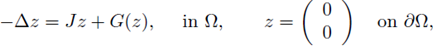
where G(z) := PF(w) = PF(P-1z).
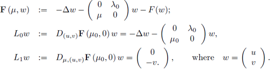
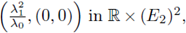
Step 2. We check that the conditions of Crandall-Rabinowitz's Theorem [24] are satisfied. Fix λ = λ0 > 0, and choose /x as the bifurcation parameter. Let σ ∈ (0,1); define
 equipped with its standard norm; E
2 is a space. Set E
0
= C
σ
(Ω) and define the operator
equipped with its standard norm; E
2 is a space. Set E
0
= C
σ
(Ω) and define the operator
 by
by
Set
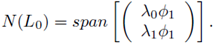
 , and P0 = P(λ0,/μ0). Observe that w ∈ N(L
0
) (where N(L
0
) is the kernel of L
0
) if, and only if,
, and P0 = P(λ0,/μ0). Observe that w ∈ N(L
0
) (where N(L
0
) is the kernel of L
0
) if, and only if,
 Therefore,
Now, we claim that
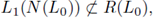 where R(L
0
) is the range of L
0.
where R(L
0
) is the range of L
0.
Indeed, assume that there exist w ∈ N(L
0
) and
 such that L1 w = L0 ψ or, equivalently by definition of L0 and L1,

Multiplying (19) on the left by P0, and denoting by
 we obtain
Multiplying the first (component) equation by ϕ1, integrating on Ω, and applying Green's formulae we obtain
Therefore a = 0. Hence, the hypotheses of Crandall Rabinowitz theorem are satisfied. Thus, there exists a neighborhood of
 and continuous functions
 such that
 with
with
 and the only nontrivial solutions of (6) for λ = λ 0 fixed, are
Observe that for s > 0 small enough,
 satisfies
 on
on
 hence
hence

Step 3. Now, we use the global bifurcation Theorem as stated by Rabinowitz [82] and as completed by Dancer [34]. Let (-Δ)-1 denote the inverse of (-Δ) with homogeneous Dirichlet boundary conditions. It follows from Schauder estimates that (-Δ)-1 maps bounded subsets of E 0 into bounded subsets of E2, which in turn are relatively compact in E0. Thus, (-Δ)-1: E0 → E0 is compact.
Observe that, fixed points of the operator (-Δ)-1 [J(.)+G(.)] corresponds to fixed points of the operator (-Δ)-1 [A(.) + F(.)], that is,

Let us keep fixed λ = λ0 > 0, and allow μ to vary. It follows from Rabinowitz's global bifurcation Theorem [82, Theorem 1.3] that there is a continuum of solutions, emanating from the trivial solution at
 which is either unbounded, or meets another bifurcation point from the trivial solution. Let

be the continuum emanating from the trivial solution at
 and solving (6) for λ = λ0 fixed. By elliptic regularity, it is known that
Considering the positive cone
 let us denote by
 Since the classical positive solutions are a priori bounded (see (18)), we have that
 is bounded. Assume that there exists
 such that
 then, either
 with (u*,v*) ≠ (0, 0). If (u*,v*) = (0, 0) then ((λ0,μ*), (u*,v*)) is a bifurcation point from the trivial solution to positive solutions. Due to the unique bifurcation point from the trivial solution to positive solutions at λ = λ0 is attained at
 if (u*,v*)
=
(0,0) then we reach a contradiction. On the other hand, if u* ≥ 0, v* ≥ 0 in Ω, (u*,v*) ≠ (0, 0), from the Maximum Principle and the Hopf Maximum Principle
if (u*,v*)
=
(0,0) then we reach a contradiction. On the other hand, if u* ≥ 0, v* ≥ 0 in Ω, (u*,v*) ≠ (0, 0), from the Maximum Principle and the Hopf Maximum Principle
 therefore
 which contradicts the hypothesis.
Remark 2.3. Let us mention that when moving λ we obtain a whole curve of nonisolated bifurcation points. If S denote the closure of the set of nontrivial solutions pairs ((λ,μ),w) of (17), and
 denote the set of bifurcation points of (17) from the trivial solution, we proved in Step 2 that the set
is a set of bifurcation points of (17) from the trivial solution. All points in
1 are nonisolated bifurcation points. Using Alexander and Antman's result [3], we can deduce that in a neighborhood of that curve, there is a bifurcating two-dimensional surface of nontrivial solution pairs ((λ,μ), (u, v)) of equation (6).
3. A priori estimates for quasilinear elliptic equations involving the p-Laplacian
Let Ω be a smooth, bounded, and strictly convex domain in ℝN
, N ≥ 2. We prove L
∞
(Ω) a priori bounds for
 weak solutions of the problem
where
 is the p-Laplace operator, 1 < p < ∞, and
(H1) f : [0, ∞) → ℝ is a locally Lipschitz continuous function with f (0) ≥ 0.
If p > 2 we also assume that f (s) > 0 if s > 0.
The equation -Δpu = f (u) is the Lp counterpart to the classical semilinear elliptic equation -Δu = f (u), and appears for instance in the theory of non-Newtonian fluids, dilatant fluids in the case p ≥ 2, pseudo-plastic fluids in the case 1 < p < 2 (see [6], [69], [70]).
If
 is a weak solution of the problem (20), then
 with τ < 1 (see [41], [60]), so we assume from the beginning a C
1 regularity for the solution, which is in general only a weak solution. A standard setting in the applications of a priori estimates to existence of solutions to elliptic problems, is the space of continuous functions. If
with τ < 1 (see [41], [60]), so we assume from the beginning a C
1 regularity for the solution, which is in general only a weak solution. A standard setting in the applications of a priori estimates to existence of solutions to elliptic problems, is the space of continuous functions. If
 then also f(u) is continuous and the solution u belongs to the space C1,T(Ω), by the cited regularity results.
Mitidieri and Pohozaev in [73], [74] proved Liouville theorems for quasilinear elliptic inequalities in ℝN involving the p-laplacian. Later, Serrin and Zou [86], and also Farina and Serrin [42], [43], proved Liouville theorems for more general operators.
With the help of the blow-up procedure, Azizieh and Clement in [9] proved a priori estimates for the equation (20) when Ω is strictly convex, 1 < p < 2 and f (u) growing not faster than a power
 at infinity, with
(see [10] for the case of systems). The exponent
 is the optimal exponent for Liouville theorems for elliptic inequalities; observe that
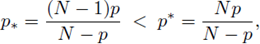
where p is the critical exponent for the Sobolev's embeddings. The restriction 1 < p < 2 depends on the fact that using a blow-up procedure and Liouville theorems on the whole space, they need to exclude concentration of maximum points of the solutions at the boundary, and they use some result proved in [29], [30] on the symmetry and monotonicity of solutions to p-Laplace equations in the singular case 1 < p < 2; these results were later extended to the case p > 2 in the papers [32], [33].
Ruiz [83] proved a priori estimates for equation more general than (20), using a different technique based among other tools on Harnack type inequalities; therein f = f (x, u, Du) can depend on x and on the gradient, for any 1 < p < N and for general domains. Once again the growth at infinity with respect to u must be less than powers with exponent
 < p* - 1.
In both papers, there is also a general discussion on how the existence of solutions follows from the a priori estimates, using some abstract results by Krasnoselskij already used in [40].
Later, Zou [92] proved Liouville theorems in half spaces that, together with the results in [84], allow him to use the blow-up method and prove a priori estimates for equations more general than (20), in case 1 < p < N; therein f = f (x, u, Du) can depend on x and on the gradient, and under various hypotheses on the nonlinearities. In particular, it is assumed that f = f (x, u, Du) grows with respect to u as a subcritical power at infinity and zero.
For monotonicity and Liouville type theorems in half spaces many other papers appeared recently (see in particular the papers of Farina, Montoro, and Sciunzi [44], [45], [46], and Farina, Montoro, Riey, and Sciunzi [47]).
In recent years, related a priori estimates for general operators were established by D'Ambrosio and Mitidieri in [26], [27].
The aim of this Section is to state a priori estimates for solutions of (20) in the case of Ω being a smooth bounded strictly convex domain, for any value of p > 1. In case 1 < p < N, f (u) is assumed to have a subcritical grow at infinity, but allowing more general functions than merely subcritical powers (see for example Corollary 1.4).
We adapt the technique introduced in [40] for the case p = 2, that allows to give the same proof in cases 1 < p < N, p = N and p > N. Of course, in the latter cases, much weaker hypotheses are needed in order to obtain the desired estimates (in particular in case p > N we only need that f (u) grows faster than up-1 at infinity, condition that for p = 2 is the superlinearity at infinity). This proofs rely deeply on the C2 regularity of solutions, which are then classical solutions, and on the W2,q estimates based on the Calderón-Zygmund and Agmon-Douglis-Nirenberg estimates [1], [2]. These estimates are not available in the singular/degenerate case p ≠ 2. We use instead regularity results for the p-laplacian (see [41], [60], [88], and gradient estimates [57], [19], [20]). There are many other tools that we had to adapt to handle in our case. We use Strong Maximum Principle and Hopf's Lemma for the p-Laplacian (see [91]), weak and strong comparison principles for the p-Laplacian (see [25], [28], [32], [33], [55], [78]), Picone's identity for the p-Laplacian ([4]), Pohozaev's identity for the p-Laplacian ([55]). Although the general theory of eigenvalues for the p-Laplacian is far from complete (see [50], [77]), the properties of the first eigenvalue are known and are the same as in the case p = 2 (see [5], [77], [61]).
All the following results are already known (see [31]):
Theorem 3.1 (Case p > N). Let Ω be a smooth bounded domain in ℝN , N ≥ 2, which is strictly convex. Assume that p > N, the condition (H1) holds and
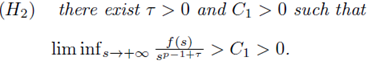
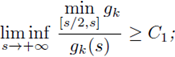
(H2) there exist T > 0 and C1 > 0 such that liminfs^+00 > d > 0.
Then, the solutions of (20) are a priori bounded in L∞: there exists a constant C, depending on p, Ω and f, but independent of the solution u, such that
 for any solution of (20).
Proof. See [31, Proof of Theorem 1.3] for a proof.
Remark 3.2. For the ordinary laplacian (p = 2), the above theorem corresponds to the case of dimension N = 1. In [40, Remark 1.3] it was observed that if N = 1, solutions are uniformly bounded under the only hypothesis of superlinearity at infinity, which corresponds for p = 2 to the hypothesis (H2) with τ = 0, and the bound from below strictly bigger than λ1 the first eigenvalue for the Laplacian operator.
We need the slightly stronger form (with T > 0 but arbitrarily small) for technical reasons (use of the Picone's Identity for the p-laplacian).
Theorem 3.3 (Case p = N). Let i be a smooth bounded domain in ℝN , N ≥ 2, which is strictly convex. Let p = N and assume that (H1) and (H2) hold, as well as
(H3) there exists C2 > 0 such that
 where
where
 is a primitive of the function f;
(H4) there exists θ > 0 such that
 (of course this is equivalent to: there exists η > 0 such that
Then, the solutions of (20) are a priori bounded in L
∞
: there exists a constant C, depending on p, Ω and f, but independent of the solution u, such that
 for any solution of (20).
Proof. See [31, Proof of Theorem 1.3] for a proof. 0
Remark 3.4. If p = 2 (the ordinary laplacian), the above theorem corresponds to the case of dimension N = 2, and in that case solutions are uniformly bounded under the only hypotheses of superlinearity together with polynomial growth at infinity (cf. [40, Theorem 1.1]). All the functions f growing polynomially at infinity are included in hypotheses (H3), and (H4).
Nevertheless, when p = N the critical embedding is of exponential type, and those hypotheses are not optimal (neither are the hypotheses in [40]), and we think that they can be improved.
The following result can be seen as the counterpart for p ≠ 2 to the results above (see [31, Proof of Theorem 1.7] for a proof).
Theorem 3.5 (Case 1 < p < N). Let Ω be a smooth bounded domain in ℝN , N ≥ 2, which is strictly convex.
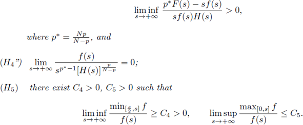
Let 1 < p < N, and assume that and (H2) hold, as well as
(H3 “) there exist a nonincreasing positive function H : [0,+∞) - ℝ such that
Then, the solutions of (20) are a priori bounded in L∞
: there exists a constant C, depending on p, Ω and the function f, but independent of the solution u, such that
 for any solution of (20).
The existence of solutions for (20) follows from the a priori estimates, with a further hypothesis about the behavior of the nonlinearity at zero.
This was proved in [40] (with the hypothesis (H0) below) for p = 2, using some variants of topological arguments, connected with theorems of Krasnoselskii [58] and Rabinowitz [81] based on degree theory. It was extended to the case of p-Laplace equations in [9], [83], [92].
It also can be adapted to our hypotheses. More precisely, the following result holds (see [31, Proof of Theorem 1.8] for a proof).
Theorem 3.6. Let us assume that the hypotheses of one of the previous theorem hold, and assume also that
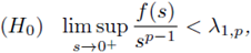
where λ1,P is the first eigenvalue for the p-Laplacian (see [31, Section 2]). (Since f (0) ≥ 0 by (H 1 ), this hypothesis implies that f (0) =0).
Then, there exists a positive solution of (20).
4. Equivalence between uniform L2* (Ω) a-priori bounds and uniform L∞(Ω) a-priori bounds for subcritical elliptic equations
We consider the existence of L ∞ (Ω) a-priori bounds for classical positive solutions to the boundary value problem

where Ω ⊂ ℝN, N > 2, is a bounded domain with C2 boundary
 . Trudinger [90] proved that any weak solution in H1(Ω) is in fact in L∞(Ω) and consequently in C∞ (Ω).
We provide sufficient conditions on f for uniform L2* (Ω) a-priori bounds to imply uniform L
∞
(Ω) a-priori bounds, where
 is the critical Sobolev exponent. The converse is obviously true without any additional hypotheses.
The ideas for the proof of the following theorem are similar to those used in [16, Theorem 1.1] (see also part I, Theorems 2.1, 2.2). Unlike the proof in [16], here we do not use Pohozaev or moving planes arguments.
Our main result is the following theorem.
Theorem 4.1. Assume that the nonlinearity f : ℝ+ → ℝ is a locally Lipschitzian function that satisfies:
(H1) There exists a constant C
0
> 0 such that
(H2) There exists a constant C
1
> 0 such that
(F)
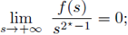 that is, f is subcritical.
Then the following conditions are equivalent:
(i) there exists a uniform constant C (depending only on Ω and f) such that for every positive classical solution u of (21),
(ii) there exists a uniform constant C (depending only on Ω and f) such that for every positive classical solution u of (21),
(iii) there exists a uniform constant C (depending only on Ω and f) such that for every positive classical solution u of (21),
Proof. All the arguments work in a similar way as in part I, Theorems 2.1, 2.1 (see also [15, proof of Theorem 1.1]). 0
In this Section, we also provide sufficient conditions for the equivalence of the existence of a uniform L2* (Ω) a priori bound with that of a uniform L∞(Ω) a priori bound for sequences of boundary value problems. In fact, we have the following theorem, which is [15, Theorem 1.2]; we include the proof by the sake of completeness.
Theorem 4.2. Consider the following sequence of BVPs

with g k: ℝ+ → ℝ locally Lipschitzian. We assume that the following hypotheses are satisfied:
(H1)k fc there, exists a uniform constant C
1 > 0 such that
(H2)k
there exists a uniform constant C
2
> 0 such that
Let {v
k
} be a sequence of classical positive solutions to
 If
If
then, the following two conditions are equivalent:
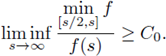
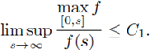
(i) there exists a uniform constant C, depending only on Ω and the sequence {gk}, but independent of k, such that for every vk > 0, classical solution to (21) k ,
(ii) there exists a uniform constant C 0 , depending only on Ω and the sequence {gk}, but independent of k, such that for every vk > 0, classical solution to (21) k ,

(iii) there exists a uniform constant C (depending only on Ω and the sequence {g k }) such that for every positive classical solution v k of (21) k ,
Hypothesis (H1)k, and (H2)k, are not sufficient for the existence of a uniform L°° a priori bound. Atkinson and Peletier in [8] show that for fε(s) = s2*-1-ε and Ω a ball in ℝ3, there exists x0 ∈ Ω and a sequence of solutions u
ε such that
 and
and
 See also Han [56], for minimum energy solutions in general domains.
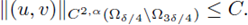
Furthermore, hypotheses (H1)k, (H2)k, and (F)k, are not sufficient for the existence of an L∞
a priori bound. In fact, at the end of this Section, we construct a sequence of BVP satisfying (H1)k, (H2)k, and (F)k, and a sequence of solutions vk such that
 Our example also shows the non-uniqueness of positive solutions.
Remark 4.3. One can easily see that condition (22), elliptic regularity and Sobolev embeddings imply that there exists a uniform constant C4 > 0 such that

for all classical positive solutions {vk} to (21)k.
The ideas for the proof of the above theorem are similar to those used in [16, Theorem 1.1] (see also Theorems 2.1, 2.1 in part I). But, unlike the proof in [16], here we do not use Pohozaev or moving planes arguments; therefore, the structure of the proof described in Subsection 1.1 of part I will start in one adaptation of Step 3.
Proof of Theorem 4.2. Clearly, condition (i) implies (ii) and (iii). By the elliptic regularity and condition (22), we have that
 Therefore,
 So, by the Sobolev embedding, we deduce that
Using similar arguments as in Theorems 2.1, 2.1 of part I and condition (F)k, one can show that (ii) and (iii) are equivalent. We shall concentrate our attention in proving that (ii) implies (i). All throughout this proof C denotes several constants independent of k.
Observe that
 From hypothesis (ii) (see (22)), there exists a fixed constant C > 0 (independent of k) such that
for k big enough, and for any q > N/2.
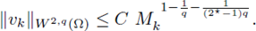
Therefore, from elliptic regularity, (see [54, Lemma 9.17]),

for k big enough.
Let us restrict q ∈ (N/2, N). From Sobolev embeddings, for 1/q* = 1/q - 1/N with q* > N, we can write

for k big enough.
From Morrey's Theorem (see [13, Theorem 9.12 and Corollary 9.14]), there exists a constant C only dependent on Ω, q and N such that

for any k.
Therefore, for all x ∈ B(x 1 , R) ⊂ Ω,

for any k.
From now on, we argue by contradiction. Let {vk} be a sequence of classical positive solutions to (21) k and assume that

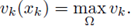
Let x k ∈ Ω be such that
Let us choose R k such that B k: = B(x k, R k) ⊂ Ω, and
and there exists yk ∈ dB k such that

Let us denote by

Therefore, we obtain

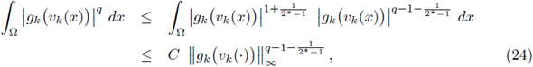
Then, reasoning as in (24), we obtain
From elliptic regularity (see (25)), we deduce
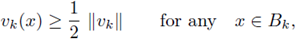
Therefore, from Morrey's Theorem (see (26)), for any x ∈ Bk),

Particularizing x = yk in the above inequality, and from (27), we obtain

which implies
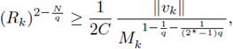
or equivalently,
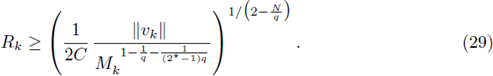
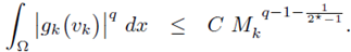
Consequently, taking into account (28),
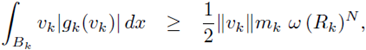
where w = wN is the volume of the unit ball in ℝN.
Due to Bk ⊂ Ω , substituting inequality (29), and rearranging terms, we obtain
At this moment, let us observe that from hypothesis (H1)k and (H2)k,
Hence, taking again into account hypothesis (H2)k, and rearranging exponents, we can assert that
Finally, from hypothesis (F)k we deduce
which contradicts (23).
4.1. Radial problems with almost critical exponent
In this Section, we build an example of a sequence of functions {gk} growing subcritically, and satisfying the hypotheses (H1)k, (H2)k, and (F)k, such that the corresponding sequence of BVP
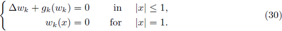
has an unbounded (in the L∞(Ω)-norm) sequence {wk} of positive solutions. As a consequence of Theorem 4.2, this sequence {wk} is also unbounded in the L2 (Ω)-norm.
Let N ≥ 3 be an integer. For each positive integer k > 2 let gk(s) =0 for
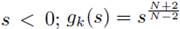 for
for
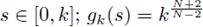 for
for
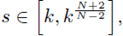 and
and
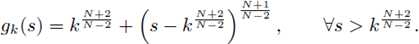
For the sake of simplicity in notation, we write gk: = g.
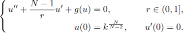
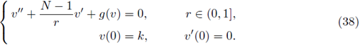
Let uk: = u denote the solution to
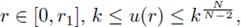
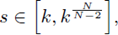
Let r1 = sup {r > 0; uk(s) ≥ k on [0, r]}. Since g ≥ 0, u is decreasing, consequently for
 and
and

so
Hence,

Thus,
 for all
 , and
, and
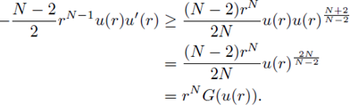
By well established arguments based on the Pohozaev identity (see [18]), we have

where
 and
and
For

Hence,

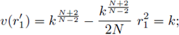
Due to Γ(s) = 0 for all s ≤ k, (33) and (34), for r ≥ r0,

From definition of r1 and (32),
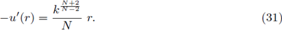
From definition of
 (see (31)), which implies
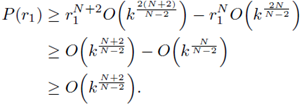
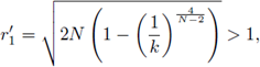
For r ≥ r1 ,
This, Pohozaev's identity, and (36) imply

Integrating on [r1, r] we have
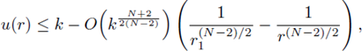
which implies that there exists k0 such that if k ≥ k0 then u(r) = 0 for some r ∈ (r1, 2r1]. Since (37), r1 = r1(k) → 0 as k → ∞.
Let v := vk denote the solution to
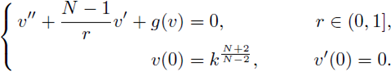
Let
 For v(r) ≥ k, integrating (31) we deduce
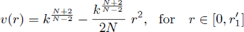
and
therefore,
so v(r) ≥ k for all r ∈ [0, 1].
Therefore, by continuous dependence on initial conditions, there exists
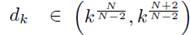 such that the solution w = w
k to
such that the solution w = w
k to
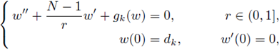
satisfies w(r) ≥ 0 for all r ∈ [0,1], and = 0. Since k may be taken arbitrarily large, and as a consequence of Theorem 4.2, we have established the following result.
Corollary 4.4. There exists a sequence of functions g k: ℝ → ℝ and a sequence {w k } of positive solutions to (30), such that each function g k grows subcritically and satisfies the hypotheses (H1) k , (H2) k and (F) k of Theorem 4.2, and the sequence {w k } of positive solutions to (30) is unbounded in the L co (Ω)-norm.
Moreover, this sequence {w k } is also unbounded in the L2* (Ω)-norm.
Let now v := v k denote the solution to
Since Γ(s) = 0 for all s ≤ k, and the solution is decreasing, by Pohozaev's identity,

Hence, if
 for some
 , then
 and the uniqueness of the solution of the IVP (38), implies v(r) = 0 for all r ∈ [0,1]. Since this contradicts v(0) = k > 0 we conclude that v(r) > 0 for all r ∈ [0,1]. Therefore, by continuous dependence on initial conditions, there exists
 such that the solution z = z
k to
such that the solution z = z
k to
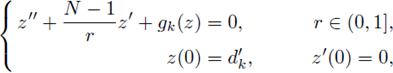
satisfies z(r) ≥ 0 for all r ∈ [0,1], and z(1) = 0.
Corollary 4.5. For any
 the BVP (30) has at least two positive solutions.
5. Asymptotics for positive radial solutions of elliptic equations approaching critical growth
Consider the classical Dirichlet boundary value problem
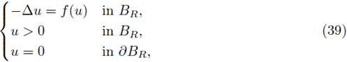
for
 in which B
R
= B
R
(0) ⊂ ℝN
, N > 2, is the open ball of radius R, and / is locally-Lipschitz in [0, ∞) and superlinear at infinity (i.e. lim inf f (u)/u > λ1 as u → ∞, where λ1 > 0 is the first eigenvalue of - Δ with Dirichlet boundary conditions). Denote by 2* := 2N/(N - 2) the critical Sobolev exponent; H
1 (Ω) is compactly embedded in Lp(Ω) if, and only if, p < 2*. The extended real number
in which B
R
= B
R
(0) ⊂ ℝN
, N > 2, is the open ball of radius R, and / is locally-Lipschitz in [0, ∞) and superlinear at infinity (i.e. lim inf f (u)/u > λ1 as u → ∞, where λ1 > 0 is the first eigenvalue of - Δ with Dirichlet boundary conditions). Denote by 2* := 2N/(N - 2) the critical Sobolev exponent; H
1 (Ω) is compactly embedded in Lp(Ω) if, and only if, p < 2*. The extended real number
 discriminates the problem (39) into three types: critical if f * ∈ (0, ∞), supercritical if f * = ∞ and subcritical if f* = 0.
Assume the nonlinearity is a pure subcritical power f (u) = u2*-1-ε, ε > 0, and Ω is a ball. Atkinson and Peletier in [8] studied the assymptotic behavior as e - 0+ of solutions to (39), and proved that
and ∀r ≠ 0,
where
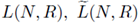 are constants only dependent on N, and R, defined by
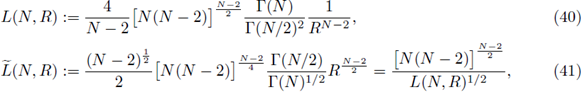
where Γ denotes the Gamma function. See also [56] with similar results for least energy solutions on general domains.
The above sections lead to a natural question: Is the lower bound on
 a technical or an intrinsic condition?
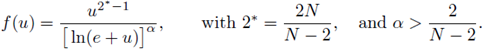
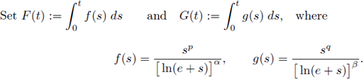
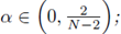
In the present Section, we focus our attention on nonlinearities

We analyze the asymptotic behavior as α → 0+ of solutions to (39). Firstly, we prove that for each
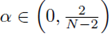 fixed, the set of positive solutions to (39) is a priori bounded.
Henceforth, the bound from below on a in [16], [17], [31], [71] are technical rather than intrinsic, at least when Ω is the open ball of radius R. Secondly, we provide estimates for the growth of uα(0) as α → 0+. We adapt for our nonlinearities, techniques introduced by Atkinson and Peletier for the case of subcritical powers in [7], [8].
Our first result is on the existence of solutions to (39), and of uniform L∞ a priori bounds for each a fixed (see [75, Proof of Theorem 1.1] for a proof).
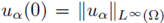
Theorem 5.1. Fix
 let f = f
α
be as in (42) and assume Ω is the open ball ofradius i . Then the following results hold:
let f = f
α
be as in (42) and assume Ω is the open ball ofradius i . Then the following results hold:
(i) There exists a radially symmetric solution to (39), u = u α (r) > 0.
(ii) There are constants A = A α (N,R), B = B α (N,R) > 0 depending only on α, N and R, such that for every u = u a > 0, radially symmetric solution to (39), we have

Our second result is an estimate of the asymptotic behavior of
 as α → 0+.
Theorem 5.2. Let f = f
α
be as in (42) with
 and Ω be the open ball of radius R. Then, there exists a constant L(N, R) > 0 only depending on N and R, such that for any u
α
= u
α
(r), radially symmetric positive solution to (39), we have
and Ω be the open ball of radius R. Then, there exists a constant L(N, R) > 0 only depending on N and R, such that for any u
α
= u
α
(r), radially symmetric positive solution to (39), we have
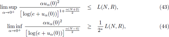
where L(N,R) is defined by (40).
Proof. See [75, Proof of Theorem 1.2].
6. Some Open Problems
- When N = 2, which is the critical nonlinearity f for having a priori bounds? (See There exists a radially symmetric s [38], There exists a radially symmetric s [39]).
- When N > 2, which is the more general subcritical nonlinearity f for having a priori bounds?
- When p = N, which is the critical nonlinearity f for having a priori bounds? (See There exists a radially symmetric s [36]).
- When N > p, which is the more general subcritical nonlinearity f for having a priori bounds? (See [36]).
See the discussion corresponding to the Lane-Emdem system (7).


