


 English (pdf)
 Article in xml format
 Article references
 Send this article by e-mail
 Cited by SciELO
  Cited by Google
  Similars in
SciELO
Similars in
SciELO  Similars in Google
 Permalink
1. Introduction
In this paper we continue the work presented in [14], extending the result to a more general and realistic scenario. That is, we find the limiting form of a Darcy-Stokes (see equations (26)) coupled system, within a saturated domain Ωє in ℝN, consisting in three parts: a porous medium Ω1 (Darcy flow), a narrow channel
 whose width is of order e (Stokes flow) and a coupling interface
 (see Figure 1 (a)). In contrast with the system studied in [14], where the interface is flat, here the analysis is extended to curved interfaces. It will be seen that the limit is a fully-coupled system consisting of Darcy flow in the porous medium Ω1 and a Brinkman-type flow on the part Γ of its boundary, which now takes the form of a parametrized N - 1 dimensional manifold.
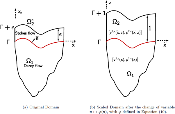
Figure 1 Figure (a) depicts the original domain with a thin channel on top, where we set the Stokes flow. Figure (b) depicts the domain after scaling by the change of variables x → φ(x), where φ is defined in Equation (10). This will be the domain of reference which is used for asymptotic analysis of the problem.
The central motivation in looking for the limiting problem of our Darcy-Stokes system is to attain a new model, free of the singularities present in (26). These are the narrowness of the channel
 (є) and the high velocity of the fluid in the channel
(є), both (geometry and velocity) with respect to the porous medium. Both singularities have a substantial negative impact in the computational implementation of the system, such as numerical instability and poor quality of the solutions. Moreover, when considering the case of curved interfaces, the geometry of the surface aggravates these effects, making even more relevant the search for an approximate singularity-free system as it is done here.
(є) and the high velocity of the fluid in the channel
(є), both (geometry and velocity) with respect to the porous medium. Both singularities have a substantial negative impact in the computational implementation of the system, such as numerical instability and poor quality of the solutions. Moreover, when considering the case of curved interfaces, the geometry of the surface aggravates these effects, making even more relevant the search for an approximate singularity-free system as it is done here.
The relevance of the Darcy-Stokes system itself, as well as its limiting form (a Darcy-Brinkman system) is confirmed by the numerous achievements reported in the literature: see [2], [4], [6] for the analytical approach, [3], [5], [9], [13] for the numerical analysis point of view, see [11], [21] for numerical experimental coupling and [12] for a broad perspective and references. Moreover, the modeling and scaling of the problem have already been extensively justified in [14]. Hence, this work is focused on addressing (rigorously) the interface geometry impact in the asymptotic analysis of the problem. It is important to consider the curvature of interfaces in the problem, rather than limiting the analysis to flat or periodic interfaces, because the fissures in a natural bedrock [where this phenomenon takes place] have wild geometry. In [7], [8] the analysis is made using homogenization techniques for periodically curved surfaces, which is the typical necessary assumption for this theory. In [17], [18] the analysis is made using boundary layer techniques, however no explicit results can be obtained, as usually with these methods. An early and simplified version of the present result can be found in [16], where incorporating the interface geometry in the asymptotic analysis of a multiscale Darcy-Darcy coupled system is done and a explicit description of the limiting problem is given.
The successful analysis of the present work is because of keeping an interplay between two coordinate systems: the Cartesian and a local one, consistent with the geometry of the interface r. While it is convenient to handle the independent variables in Cartesian coordinates, the asymptotic analysis of the flow fields in the free fluid region
 is more manageable when decomposed in normal and tangential directions to the interface (the local system). The a-priori estimates, the properties of weak limits, as well as the structure of the limiting problem will be more easily derived with this double bookkeeping of coordinate systems, rather than disposing of them for good. It is therefore a strategic mistake (not a mathematical one, of course) to seek a transformation flattening out the interface, as it is the usual approach in traces' theory for Sobolev spaces. The proposed method is significantly simpler than other techniques and it is precisely this simplicity which permits to obtain the limiting form explicit description for a problem of such complexity, as a multiscale coupled Darcy-Stokes.
Notation
We shall use standard function spaces [see [1], [20]). For any smooth bounded region G in ℝN with boundary ∂G, the space of square integrable functions is denoted by L2(G) and the Sobolev space H
1(G) consists of those functions in L2(G) for which each of its first-order weak partial derivatives belongs to L
2(G). The trace is the continuous linear function γ : H1(G) - L
2(∂G) which agrees with the restriction to the boundary on smooth functions, i.e.,
 Its kernel is
 The trace space is
 the range of γ endowed with the usual norm from the quotient space
 and we denote by H-1/2(∂G) its topological dual. Column vectors and corresponding vector-valued functions will be denoted by boldface symbols, e.g., we denote the product space [L2(G)]N by L2(G) and the respective N-tuple of Sobolev spaces by
 Each w ∈ L
2(G) has gradient
Each w ∈ L
2(G) has gradient
 furthermore we understand it as a row vector. We shall also use the space Hdiv(G) of vector functions w ∈ L2(G) whose weak divergence ∇ • w belongs to L2(G). The symbol
 stands for the unit outward normal vector on ∂G. If w is a vector function on ∂G, we indicate its normal component by
 and its normal projection by
 The tangential component is denoted by
 The notations w
N, wT indicate respectively, the last component and the first N - 1 components of the vector function w in the canonical basis. For the functions w ∈ Hdiv(G), there is a normal trace defined on the boundary values, which will be denoted by
The notations w
N, wT indicate respectively, the last component and the first N - 1 components of the vector function w in the canonical basis. For the functions w ∈ Hdiv(G), there is a normal trace defined on the boundary values, which will be denoted by
 For those w ∈ G H
1(G) this agrees with
For those w ∈ G H
1(G) this agrees with
 Greek letters are used to denote general second-order tensors. The contraction of two tensors is given by
 For a tensor-valued function k on ∂G, we denote the normal component (vector) by
 and its normal and tangential parts by
 respectively. For a vector function w ∈ H1(G), the tensor
 is the gradient of w and the tensor (£(w)) = ^(ff^ + is the symmetric gradient.
The set
 indicates the standard canonical basis in ℝN. For a column vector x = (x
1
,..., x
N-1, x
N) ∈ ℝN we denote by
indicates the standard canonical basis in ℝN. For a column vector x = (x
1
,..., x
N-1, x
N) ∈ ℝN we denote by
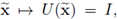
 the vector in ℝN-1 consisting of the first N - 1 components of x. In addition, we identify ℝN-1 x {0} with ℝN-1 by
 The operators
 denote respectively the ℝN-1-gradient and the ℝN-1-divergence in the first N - 1-canonical directions, i.e.,
 moreover, we regard ∇T as a row vector. Finally,
 denote the corresponding operators written as column vectors.
Remark 1.1. It shall be noticed that different notations have been chosen to indicate the first N - 1 components: we use
 for a vector variable as x, while we use wT for a vector function w (or the operator ∇T
, ∇ ). This difference in notation will ease keeping track of the involved variables and will not introduce confusion.
for a vector variable as x, while we use wT for a vector function w (or the operator ∇T
, ∇ ). This difference in notation will ease keeping track of the involved variables and will not introduce confusion.
Preliminary Results
We close this section recalling some classic results.
Lemma 1.2. Let G ⊂ ℝN
be an open set with Lipschitz boundary, and
 be the unit outward normal vector on ∂G. Let the normal trace operator
 be defined by

For any g ∈ H
-1/2(∂G) there exists u G Hdiv(G) such that
 on ∂G and
 with K depending only on the domain G. In particular, if g belongs to L
2(∂G), the function
u
satisfies the estimate
with K depending only on the domain G. In particular, if g belongs to L
2(∂G), the function
u
satisfies the estimate
Proof. See Lemma 20.2 in [19].
Next we recall a central result to be used in this work
Theorem 1.3. Let X, Y, X', Y' be Hilbert spaces and their corresponding topological duals. Let A: X → X', B : X → Y', C : Y → Y' be linear and continuous operators satisfying the following conditions
I. A is non-negative and X-coercive on ker(B);
II. B satisfies the inf-sup condition

III. C is non-negative and symmetric.
Then, for every F 1 ∈ X' and F 2 ∈ Y', the problem (3) below has a unique solution (x, y) ∈ X x Y:

Moreover, the solution satisfies the estimate

for a positive constant c depending only on the preceding assumptions on A, B, and C.
Proof. See Section 4 in [10].
2. Geometric setting and formulation of the problem
In this section we introduce the Darcy-Stokes coupled system when the interface is curved, analogous to the one presented in [14]. We begin with the geometric setting
2.1. Geometric setting and change of coordinates
We describe here the geometry of the domains to be used in the present work; see Figure 1 (a) for the case N =2. The є-domain
 is composed of two disjoint bounded open sets Ω1 and
 in ℝN sharing a common interface
 The domain Ω1 is the porous medium and
 is the free fluid region. For simplicity we have assumed that the domain
is a cylinder defined by the interface Γ and a small height є > 0. It follows that the interface must verify specific requirements for a successful analysis
is the free fluid region. For simplicity we have assumed that the domain
is a cylinder defined by the interface Γ and a small height є > 0. It follows that the interface must verify specific requirements for a successful analysis
Hypothesis 1. There exist G0, G bounded open connected domains in ℝN-1 such that cl(G) ⊂ G0, and a function ζ : G0 → ℝ, in C2(G0), such that the interface Γ can be described by

That is, Γ is aparametrized N - 1 manifold in ℝN. In addition, the domain
is described by

Remark 2.1. I. Observe that the domain G is the orthogonal projection of the open surface Γ ⊆ ℝN into ℝN-1.
II. Notice that due to the properties of ζ it must hold that if
 is the upwards unitary vector, orthogonal to the surface Γ, then

Here
 is the last element of the standard canonical basis in ℝN
For simplicity of notation in the following we write
In order to conduct the asymptotic analysis of the coupled system, a domain of reference n needs to be settled (see Figure 1 (b)). Therefore, we adopt a bijection between domains and account for the changes in the differential operators.
Definition 2.2. Let
 be the change of variables defined by
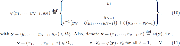
where
 are the standard canonical basis in ℝN.
Remark 2.3. Observe that
 is a bijective map (see Figure 1 (b)).
Gradient operator
Denote by y, x∇ the gradient operators with respect to the variables y and x respectively. Due to the convention of equation 9 above, a direct computation shows that these operators satisfy the relationship
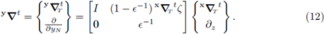
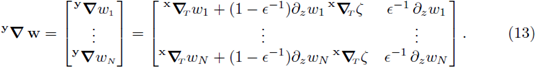
In the block matrix notation above, it is understood that I is the identity matrix in
 are vectors in ℝN-1 and
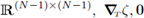
 In order to apply these changes to the gradient of a vector function w, we recall the matrix notation
Reordering we get
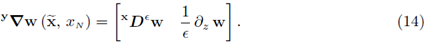
Here, the operator x£)e is defined by

i.e.,
 it is introduced to have a more efficient notation. In the next section we address the interface conditions.
Divergence operator
Observing the diagonal of the matrix in (13) we have

Remark 2.4. The prescript indexes y, x written on the operators above were used only to derive the relation between them; however, they will be dropped once the context is clear.
Local vs global vector basis
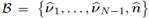
It shall be seen later on, that the velocities in the channel need to be expressed in terms of an orthonormal basis B, such that the normal vector
 belongs to B, and the remaining vectors are locally tangent to the interface Γ. Since ζ : G → ℝ is a C2 function, it follows that
 is at least C1.
Definition 2.5. Let
 be the standard canonical basis in ℝN. For any
 be an orthonormal basis in ℝN. Define the linear map
 by
by

We say the map
 is a stream line localizer if it is of class C1. In the sequel we write it with the following block matrix notation:

Here, the indexes T and N stand for the first N - 1 components and the last component of the vector field. The indexes tg and
indicate the tangent and normal directions to the interface Γ.
Remark 2.6. I. Since ζ is bounded an C2(C), clearly for each
 a basis
 can be chosen so that
 is C1. In the following it will be assumed that U is a stream line localizer.
II. Notice that by definition
 is an orthogonal matrix for all
 .
.
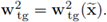
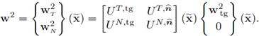
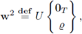
Next, we express the velocity fields w2 in terms of the normal and tangential components, using the following relations:
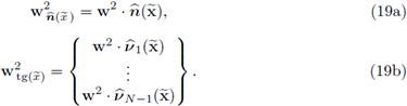
Clearly, if
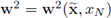 is expressed in terms of the canonical basis, the relationship between velocities is given by
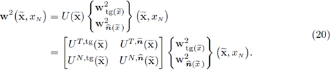
Remark 2.7. We stress the following observations
I. The procedure above does not modify the dependence of the variables; only the way velocity fields are expressed as linear combinations of a convenient (stream line) orthonormal basis.
II. The fact that U is a smooth function allows to claim that
 belongs to
 and
and
III. In order to keep notation as light as possible, the dependence of the matrix U with respect to
 , as well as the normal and tangential directions
, tg will be omitted whenever is not necessary to write explicitly these parameters.
, as well as the normal and tangential directions
, tg will be omitted whenever is not necessary to write explicitly these parameters.
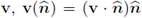
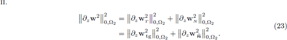
IV. Recall that for any vector field
 denotes its normal projection on the direction
 , while v(tg) = v - v(
), i.e., the component orthogonal to
(and tangent to Γ). Considering the previous, given any two flow fields u
2, w
2, the following isometric identities hold:
, while v(tg) = v - v(
), i.e., the component orthogonal to
(and tangent to Γ). Considering the previous, given any two flow fields u
2, w
2, the following isometric identities hold:
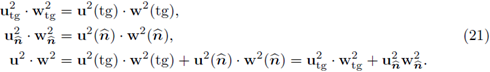
Proposition 2.8. Let w2 ∈ H1(Ω2);
and let
 be as defined in (19). Then,
Proof. I. It suffices to observe that the orthogonal matrix U defined in (20) is independent from z.
II. Due to (22), we have
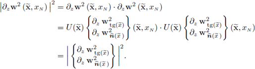
The last equality holds true because the matrix U ( ) is orthogonal at each point
  , therefore it is an isometry in the Hilbert space ℝN endowed with the standard inner product. Recalling that
 for all
 the result follows.
2.2. Interface conditions and the strong form
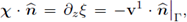
The interface conditions need to account for stress and mass balance. We start decomposing the stress in its tangential and normal components; the former is handled by the Beavers-Joseph-Saffman (24a) condition and the latter by the classical Robin boundary condition (24b); this gives
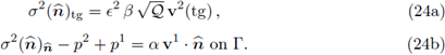
In the expression (24a) above, e2 is a scaling factor introduced to balance out the geometric singularity coming from the thinness of the channel. In addition, the coefficient α ≥ 0 in (24b) is the fluid entry resistance.
Next, recall that the stress satisfies
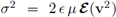 (where the scale e is introduced according to the thinness of the channel and μ > 0 is the shear viscosity of the fluid; see also Hypothesis 2) and that ∇· v2 =0 (since the system is conservative); then we have

Replacing in the equations (24) we derive the following set of interface conditions:

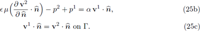
The condition (25c) states the fluid flow (or mass) balance.
With the previous considerations, the Darcy-Stokes coupled system in terms of the velocity v and the pressure p is given by
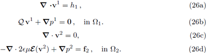
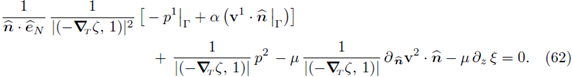
Here, equations (26a), (26b) correspond to the Darcy flow filtration through the porous medium, while equations (26c) and (26d) stand for the Stokes free flow. Finally, we adopt the following boundary conditions:
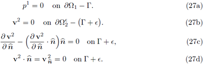
The system of equations (26), (27) and (25) constitute the strong form of the Darcy-Stokes coupled system.
Remark 2.9. i. For a detailed exposition on the system's scaling, namely, the fluid stress tensor
 and the Beavers-Joseph-Saffman condition (24a), together with the formal asymptotic analysis, we refer to [15].
II. A deep discussion on the role of each physical variable and parameter in equations (26), as well as the meaning of the boundary conditions (27), can be found in Sections 1.2, 1.3 and 1.4 in [14].
2.3. Weak variational formulation and a reference domain
In this section we present the weak variational formulation of the problem defined by the system of equations (26), (27) and (25), on the domain Ωє. Next, we rescale
 to get a uniform domain of reference. We begin defining the function spaces where the problem is modeled.
Definition 2.10. Let
 be as introduced in Section 2.1; in particular, Ω2 and Γ satisfy Hypothesis 1. Define the spaces

endowed with their respective natural norms. Moreover, for є =1 we simply write X, X2 and Y.
In order to attain well-posedness of the problem, the following hypothesis is adopted.
Hypothesis 2. It will be assumed that μ, > 0 and that the coefficients β, α are non-negative and bounded almost everywhere. Moreover, the tensor
 is elliptic, i.e., there exists a positive constant CQ such that

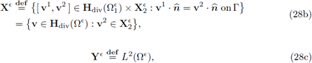
Theorem 2.11. Consider the boundary-value problem defined by the equations (26), the interface coupling conditions (25) and the boundary conditions (27); then,
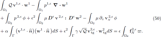
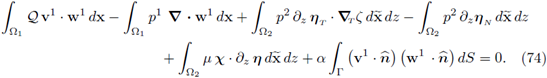
I. A weak variational formulation of the problem is given by
II. The problem (29) is well-posed.
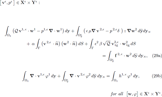
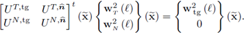
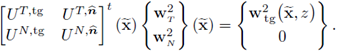
III. The problem (29) is equivalent to
Proof. I. See Proposition 3 in [14]. We simply highlight that the term
 has been replaced by
 due to the isometric identities [21].
II. See Theorem 6 in [14]. The technique identifies the operators A, B, C in the variational statements (29a) and (29b), then it verifies that these operators satisfy the hypotheses of Theorem 1.3; this result delivers well-posedness.
III. A direct substitution of the expressions (14) and (16) in the statements (29), combined with the definition (15) yields the system (30). (Also notice that the determinant of the matrix in the right hand side of the equation (14) is equal to є
-1
.) Finally, observe that the boundary conditions of space
 defined in (28a) are transformed into the boundary conditions of X2 because none of them involve derivatives.
Remark 2.1f. In order to prevent heavy notation, from now on we denote the volume integrals by
 F dx and
 We will use the explicit notation
 only when specific calculations are needed. Both notations will be clear from the context.
3. Asymptotic analysis
In this section, we present the asymptotic analysis of the problem, i.e., we obtain a-priori estimates for the solutions ((vє, pє) : є > 0), derive weak limits and conclude features about them (velocity and pressure). We start recalling a classical space.
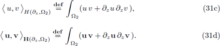
Definition 3.1. Let Ω2 be as in Definition 1 and define the Hilbert spaces
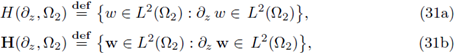
endowed with the corresponding inner products
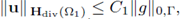
Lemma 3.2. 1. Let H(∂z, Ω2) be the space introduced in Definition 3.1; then, the trace map
 from H(∂z, Ω2) to L
2(Γ) is well-defined. Moreover, the following Poincaré-type inequalities hold in this space:
from H(∂z, Ω2) to L
2(Γ) is well-defined. Moreover, the following Poincaré-type inequalities hold in this space:
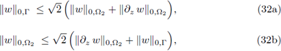
for all w ∈ H(∂z, Ω2).
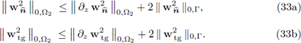
II. Let H(∂z, Ω2) be the vector space introduced in Definition 3.1; then, for any w ∈ H(∂z, Ω2) the estimates analogous to (32) hold.
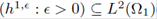
III. Let w2 ∈ H
1(Ω2) ⊂ H(∂z, Ω2) and let
 be as defined in (19); then,
Proof. I. The proof is a direct application of the fundamental theorem of calculus on the smooth functions C ∞ (Ω2), which is a dense subspace in H(∂z, Ω2).
II. A direct application of equations (32) on each coordinate of w ∈ H(∂z, Ω2) delivers the result.
III. It follows from a direct application of (i) and (ii) on
 respectively.
Next we show that the sequence of solutions is globally bounded under the following hypothesis.
Hypothesis 3. In the following, it will be assumed that the sequences
 and
and
 are bounded, i.e., there exists C > 0 such that

Theorem 3.3 (Global a-priori Estimate). Let ([vє , p є]: e > 0) ⊆ X x Y be the sequence of solutions to the є-Problems (30). There exists a constant K > 0 such that

Proof. Set w = vє in (30a), φ = p є in (30b) and add them together. (Observe that the mixed terms were canceled out on the diagonal.) Next, apply the Cauchy-Bunyakowsky-Schwartz inequality to the right hand side and recall the Hypothesis 2; this gives
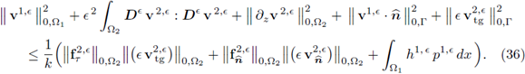
We continue focusing on the last summand of the right hand side in the expression above, i.e.,
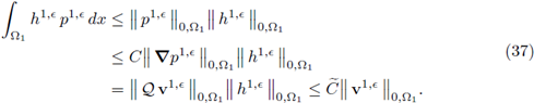
The second inequality holds due to Poincaré's inequality, given that p1,є = 0 on ∂Ω1
- Γ, as stated in Equation (27a). The equality holds due to (26b). The third inequality holds because the tensor
 and the family of sources
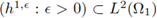 are bounded as stated in Hypothesis 2 and Hypothesis 3 (Equation (34)), respectively. Next, we control the L2(Ω2)-norm of v2,є. Since v2,є ∈ H1(Ω2) ⊂ H(∂z, Ω2), the estimates (33) apply; combining them with (37) and the bound (34) (from Hypothesis 3) in Inequality (36) we have
Here, the last inequality is due to the equality
 Next, using the equivalence of norms
 for 4-D vectors in the previous expression yields
From the expression above, the global Estimate (35) follows.
In the next subsections we use weak convergence arguments to derive the functional setting of the limiting problem (see Figure 2), for the structure of the limiting functions.
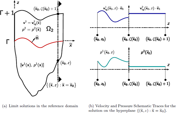
Figure 2 Figure (a) depicts the dependence of the limit solution [v, p], for both regions Ω1, Ω2 and a generic hyperplane
 Figure (b) shows plausible schematics for traces of the velocity and pressure restricted to the hyperplane
 depicted in Figure (a).
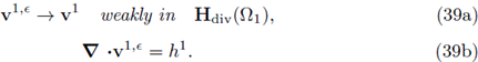
Corollary 3.4 (Convergence of the Velocities). Let ([vє, pє] : є > 0) ⊆ X x Y be the sequence of solutions to the e-Problems (30). There exists a subsequence, still denoted (vє: є > 0) , for which the following holds:
I. There exist v1 є Hd¡v(Ω1) such that
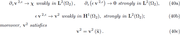
II. There exist
 and v2 ∈ H1(Ω2) such that
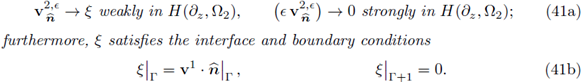
III. There exists ξ ∈ H(∂z, Ω2) such that
IV. The following properties hold:

Proof. I. (The proof is identical to part (i) of Corollary 11 in [14]; we write it here for the sake of completeness.) Due to the global a-priori estimate (35), there must exist a weakly convergent subsequence and a limit v1 ∈ Hdiv(Ω1) such that (39a) holds only in the weak L2(Ω1)-sense. Because of the hypothesis 3 and the equation (26c), the sequence
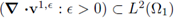 is bounded. Then, there must exist yet another subsequence, still denoted the same, such that (39a) holds in the weak Hdiv(Ω1)-sense. Now, recalling that the divergence operator is linear and continuous with respect to the Hdiv-norm, the identity (39b) follows.
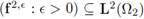
II. From the estimate (35), it follows that (∂z v2,є: є > 0) is bounded in L2(Ω2). Then, there exists a subsequence (still denoted the same) and
such that (∂z v2,є: є > 0) and (∂z(є v2,є) : є > 0) satisfy the statement (40a). Also from (35) the trace on the interface
 is bounded in L2(Γ). Applying the inequality (32b) for vector functions, we conclude that (є v 2,є: є > 0) is bounded in L2(Ω2) and consequently in H(∂z, Ω2). Then, there must exist v2 ∈ H(∂z, Ω2) such that

Also, from the strong convergence in the statement (40a), it follows that v2 is independent from z, i.e., (40c) holds.
Again, from (35) we know that the sequence (є D є v 2,є: є > 0) is bounded in L2(Ω2). Recalling the identity (15) we have that the expression

is bounded. In the equation above, the left hand side and the second summand of the right hand side are bounded in L2(Ω2); then we conclude that the first summand of the right hand side is also bounded. Hence, we have
 is bounded in L2(Ω2), and therefore the sequence (є v 2,є: є > 0) is bounded in H1(Ω2); consequently, the statement (40b) holds.
III. Since
 is bounded, in particular
 is also bounded. From (35), we know that
 is bounded and again, due to Inequality (32b), we conclude that
 is bounded. Then, the sequence
 is bounded in H(∂z, Ω2); consequently, there must exist a subsequence (still denoted the same) and a limit ξ ∈ H(∂z, Ω2), such that
 and
and
 satisfy the statement (41a). From here it is immediate to conclude the relations (41b).
IV. Since
 and due to (43), we conclude that
 Finally, due to (40), we have that
 and the proof is complete.
Theorem 3.5 (Convergence of Pressures). Let ([v є , p є]: є > 0) ⊆ X x Y be the sequence of solutions to the e-Problems (30). There exists a subsequence, still denoted (p є : є > 0), verifying the following:
I. There exists p1 ∈ H1(Ω1) such that
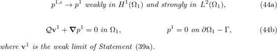
II. There exists p 2 ∈ L 2(Ω2) such that

III. The pressure p = [p1, p2] belongs to L 2(Ω).
Proof. I. (The proof is identical to part (i) Lemma 11 in [14]; we write it here for the sake of completeness.) Due to (16b) and (36) it follows that
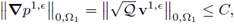
where C is an adequate positive constant. From (11a), the Poincaré inequality gives the existence of a constant
 satisfying

Therefore, the sequence (p
1.є
: є > 0) is bounded in H and the convergence statement (44a) follows directly. Again, given that p
1.є satisfies the Darcy equation (16b) and that the gradient ∇ is linear and continuous in H1(Ω1), the equality
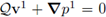 in (44b) follows. Finally, since
 for every element of the weakly convergent subsequence, and the trace map
 is linear, it follows that p1 satisfies the boundary condition in (44b).
II. In order to show that the sequence (p2,є
: є > 0) is bounded in L
2(Ω2), take any
 and define the auxiliary function

Since ζ ∈ C
2(G), it is clear that
 and
and
 Hence, the function
 belongs to X2; moreover,
Here, the second inequality follows from the first one and due to the estimate (31a). Next, observe that
 then, Lemma 1.1 gives the existence of a function w1 ∈ Hdiv (Ω1) such that
Here, the last inequality holds because
 Hence, the function
 belongs to the space X. Testing (30a) with w yields
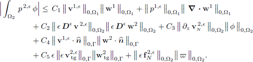
Applying the Cauchy-Bunyakowsky-Schwarz inequality to the integrals, and reordering, we get
We pursue estimates in terms of
 to that end we first apply the fact that all the terms involving the sol|ution on the right hand side, i.e.,
 are bounded. In addition, the forcing term
 is bounded. Replacing the norms of the aforementioned terms by a generic constant on the right hand side we have
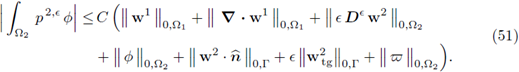
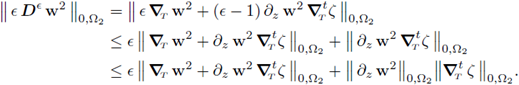
In the expression above the first summand of the second line needs further analysis. We have
Combining (48) with the expression above, we conclude

Introducing the latter estimate in the inequality (51), the first two summands on the right hand side of the first line are bounded by a multiple of
 due to (49). The second and third summands on the second line are trace terms which are also controlled by a multiple of
, due to (48). The fourth summand on the second line is trivially controlled by
due to (49). The second and third summands on the second line are trace terms which are also controlled by a multiple of
, due to (48). The fourth summand on the second line is trivially controlled by
 because of its construction. Combining all these observations with (52), we get

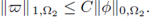
where C > 0 is a new generic constant. Taking upper limit as є → 0 in the previous expression gives

The above holds for any
 then, the sequence (p 2,є: є > 0 ) ⊂ L2(Ω2) is bounded and, consequently, the convergence statement (45) follows.
III. From the previous part, it is clear that the sequence ([p1,є, p2,є] : є > 0) is bounded in L2(Ω); therefore, p also belongs to L2Ω), which completes the proof.
Remark 3.6. Notice that the upwards normal vector
 orthogonal to the surface Γ is given by the expression

and the normal derivative satisfies

We use the identities above to identify the dependence of x, ξ and p2 (see Figure 2 above).
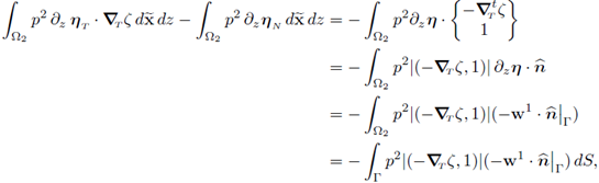
Theorem 3.7. Let x, ξ be the higher order limiting terms in Corollary 3.4 (ii) and (iii), respectively. Let p 2 be the limit pressure in Ω2 in Lemma 3.5 (ii). Then,
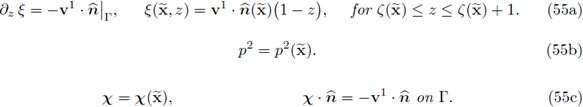
In particular,

Proof. Take Ф = (0, φ 2) ∈ Y, test (30b) and reorder the summands conveniently; we have
Letting e ↓ 0 in the expression above we get

Recalling Equation (40c) we have that ∂z v2 = 0; hence,
Since the above holds for all
 it follows that
where c is a constant. In the previous expression we observe that two out of three terms are independent from z; then it follows that the third term is also independent from z. Since the vector
 is independent from z, we conclude that
 This, together with the boundary conditions (41b), yield the second equality in (55a).
Take
 for each i =1, 2,..., N; build the "antiderivative"
 of ϕ
i using the rule (47), and define
of ϕ
i using the rule (47), and define
 Use Lemma 1.2 to construct w1 ∈ Hdiv(Ω1) such that
 and
and

therefore,
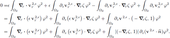
 Test (30a) with w and regroup the higher order terms; we have
The limit of all the terms in the expression above when e ↓ 0 is clear except for one summand, which we discuss independently; i.e.,
In the latter expression, the first summand clearly tends to zero when e ↓ 0. Therefore, we focus on the second summand:
All the terms in the right hand side can pass to the limit. Recalling the statement (40a), we conclude that
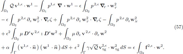
Letting e ↓ 0 in (57), and considering the equality above, we get
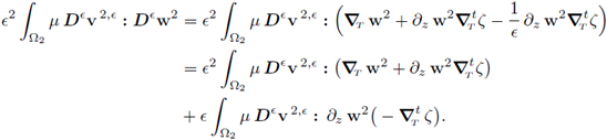
We develop a simpler expression for the sum of the fourth, fifth and sixth terms:
Here
 is the normal derivative defined in the identity (54b). We introduce the previous equality in (58); this yields
Next, we integrate by parts the second summand in the first line, add it to the first summand and recall that
 by construction. Hence,
In the expression above we develop the surface integrals as integrals over the projection G of Γ on ℝN-1; this gives
Recalling that
 the latter equality becomes in
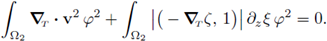
Introducing the previous in (60), we have
Since the above holds for all
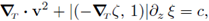
 it follows that
In order to get the normal balance on the interface w(e coul)d repeat the previous strategy, but with a quantifier
 satisfying
 i.e., such that it is parallel to the normal direction. This would be equivalent to replace ψ by
 n in all the previous equations. Consequently, in order to get the normal balance, it suffices to apply
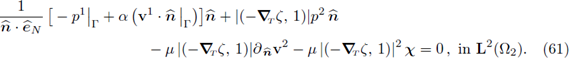
 Equation (61); such operation yields:
In the last expression the identity (42) has been used. Also notice that all the terms are independent from z, then the equation (55b) follows. Consequently, all the terms but the last in (61) are independent from z; therefore we conclude that X is independent from z. Recalling (42) and (55a), the second equality in (55c) follows and the proof is complete.
4. The limiting problem
In this section we derive the form of the limiting problem and characterize it as a Darcy-Brinkman coupled system, where the Brinkman equation takes place in a parametrized (N - 1)-dimensional manifold of ℝN. First, we need to introduce some extra hypotheses to complete the analysis.
Hypothesis 4. In the following, it will be assumed that the sequence of forcing terms
 and
and
 are weakly convergent, i.e., there exist f2 ∈ L2(Ω2) and h1 ∈ L2(Ω1) such that

4.1. The tangential behavior of the limiting problem
Recalling (40c) and (42), clearly the lower order limiting velocity has the structure
The above motivates the following definition.
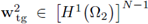
Definition 4.1. Let
 be the matrix-valued map introduced in Definition 2.5. Define the space Xtg ⊆ X2 by

endowed with the H1(Ω2)-norm.
We have the following result:
Lemma 4.2. The space Xtg ⊂ X2 is closed.
Proof. Let
 and w2 ∈ X2 be such that
 W( e) must show that w2 ∈ Xtg. First, notice that the convergence in X2 implies
 Recalling (20) and the fact that
 ) is orthogonal, we have
In the identity above, we observe that
 ) are convergent in the H1-norm and that the orthonormal matrix U has differentiability and boundedness properties. Therefore, we conclude that
 is convergent in the H1-norm, and denote the limit by
 Now take the limit in the expression above in the L2-sense; given that there are no derivatives involved, we have
Observe that the latter expression implicitly states that
 Finally, applying once more the inverse matrix, we have
Here the equality is in the L2-sense. However, we know that
 therefore the equality holds in the H1 -sense too, i.e. Xtg is closed as desired.
Next we use space Xtg to determine the limiting problem in the tangential direction.
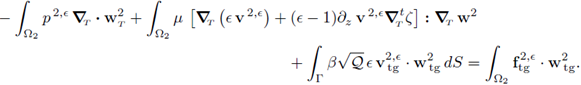
Lemma 4.3 (Limiting tangential behavior's variational statement). Let v2 be the limit found in Theorem 3.4 (ii). Then, the following weak variational statement is satisfied:
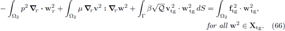
Proof. Let w2 ∈ Xtg; then w = (0, w2) ∈ X; test (30a) with w and get

Divide the whole expression over e, expand the second summand according to the identity (15) and recall that ∂z w2 = 0; this gives
Letting e ↓ 0, the limit v2 meets the condition
We modify the higher order term using the property ∂z w2 = 0:

Recall that
 , because w2 ∈ Xtg; then
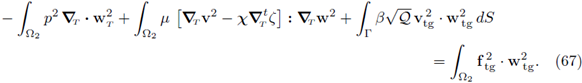
 Replacing the above expression in (67), the statement (66) follows because all the previous reasoning is valid for w2 ∈ Xtg arbitrary.
4.2. The higher order effects and the limiting problem
The higher order effects of the e-problem have to be modeled in the adequate space; to that end we use the information attained. We know the higher order term x satisfies the condition (55c) and it belongs to L2(Ω2). This motivates the following definition:
Definition 4.4. Define
I. The subspace

endowed with its natural norm.
II. The space of limit normal effects in the following way:

endowed with its natural norm

Remark 4.5. I. It is direct to prove that
 is closed.
II. Observe that, due to its structure, the component η of an element in
can be completely described by its normal trace on Γ, i.e., the norm

is equivalent to the norm (69b). This feature will permit the dimensional reduction of the limiting problem formulation later on (see Section 5.2).
III. Let v1 and ξ be the limits found in the statements (39a) and (41a), respectively. The function [v1, ξ] belongs to
, with
This was one of the motivations behind the definition of the space
 above.
iv. The information about the higher order term x is complete only in its normal direction
 Furthermore, the facts that x depends only on
 (see Equation (55c)) and that
 show that only information corresponding to the normal component of x will be preserved by the modeling space
, while the tangential component of the higher order term x(tg) will be given away for good. It is also observed that most of the terms involving the presence of x require only its normal component, e.g.
show that only information corresponding to the normal component of x will be preserved by the modeling space
, while the tangential component of the higher order term x(tg) will be given away for good. It is also observed that most of the terms involving the presence of x require only its normal component, e.g.
 in the third summand of the variational statement (66). This was the reason why the space
excludes tangential effects of the higher order term.
in the third summand of the variational statement (66). This was the reason why the space
excludes tangential effects of the higher order term.
Before characterizing the asymptotic behavior of the normal flux we need a technical lemma.
Lemma 4.6. The subspace
 is dense in
.
is dense in
.
Proof. Consider an element
 then η
tg = 0T, and
then η
tg = 0T, and
 is completely defined by its trace on the interface Γ. Given e > 0, take
 such that
 Now extend the function to the whole domain using the rule
 then
then
 From the construction of
  we know that
 Define
 due to Lemma 1 there exists u ∈ Hdiv(Ω1) such that
 on
on
 on ∂Ω1 - Γ and
 with C1 depending only on Ω1. Then, the function w1 + u is such that
 and
and
 Moreover, defining
we notice that the function (w1 +u, w2) belongs to
 Due to the previous observations we have

Given that the constants depend only on the domains Q
i and Q2, it follows that
 is dense in
.
is dense in
.
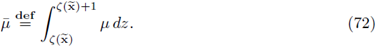
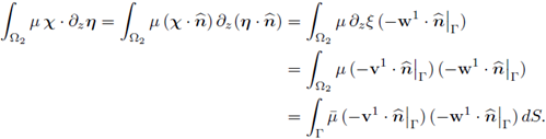
Definition 4.7. Let μ be the shear viscosity of the fluid, and define its average in the z-direction by
Lemma 4.8 (Limiting normal behavior's variational statement). Let v 1 , v2 be the limits found in Corollary 3.4, and let p 1 , p 2 be the limits found in Theorem 3.5. Then, the following variational statement is satisfied:
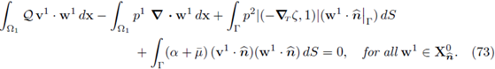
Here,
 is the averaged viscosity introduced in Definition 4-7.
Proof. Test (30a) with
 and let є → 0; this gives
Notice that the third and fourth summands in the expression above can be written as
where the second equality holds by the definition of  and the last equality holds since p2 is independent from z (see Equation (55b)). Next, recalling the identities (42), (55a) and (55c), observe that
Replacing the last two identities in (74), we conclude that the variational statement (73) holds for every test function in
 . Since the bilinear form of the statement is continuous with respect to the norm
 and
is dense in
and
is dense in
 , it follows that the statement holds for every element w ∈
.
, it follows that the statement holds for every element w ∈
.
4.3. Variational formulation of the limit problem
In this section we give a variational formulation of the limiting problem and prove it is well-posed. We begin characterizing the limit form of the conservation laws.
Lemma 4.9 (Mass conservation in the limit problem). Let v 1 , v2 be the limits found in Theorem 3.4; then,
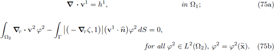
Proof. Take Ф = (φ 1,0) ∈ Y, test (30b) and let є ↓ 0; we have

The statement above implies (75a).
For the variational statement (75b), first recall the dependence of the limit velocity given in equation (55b). Hence, consider Ф = (0, φ
2) G Y such that
 test (30b) and regroup terms using (54a). The previous yields

Next, let є ↓ 0 and get

In the expression above, recall that
 and the identity (55a); then, the statement (75b) follows.
Next, we introduce the function spaces of the limiting problem:
Definition 4.10. Define the space of velocities by

endowed with the natural norm of the space
 Define the space of pressures by

endowed with its natural norm.
Theorem 4.11 (Limiting problem variational formulation). Let v 1 , v 2 be the limits found in Corollary 3.4, and let p 1 , p 2 be the limits found in Theorem 3.5. Then, they satisfy the following variational problem:
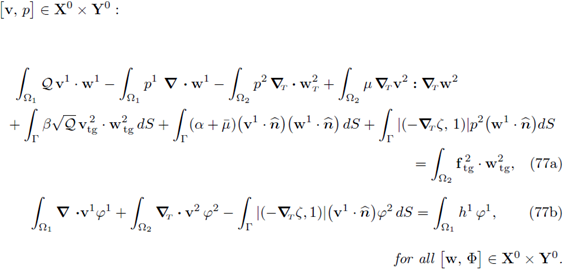
Moreover, the problem (77) is well-posed. (Here,
 is the averaged viscosity introduced in Definition 4.7.)
Proof. Since [v, p] satisfies the variational statements (66), (73), (75a), (75b) as shown in Lemmas 4.3, 4.8 and 4.9, respectively, it follows that [v, p] satisfies the problem (77) above.
In order to show that the problem is well-posed w(e prove)continuous depen(dence )of the solution with respect to the data. Test (77a) with v1, v2 and (77b) with (p1, p2), add them together and get
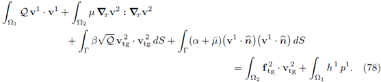
Applying the Cauchy-Bunyakowsky-Schwarz inequality to the right hand side of the expression above, and recalling that
 is constant in the z-direction, we get
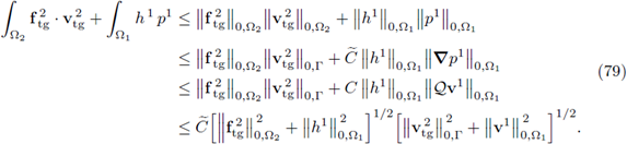
Here, the second and third inequalities holds because p1 satisfies respectively the drained boundary conditions (Poincaré's inequality applies) and the Darcy's equation as stated in (44a). Finally, the fourth inequality is a new application of the Cauchy-Bunyakowsky-Schwarz inequality for 2-D vectors. Introducing (79) in (78), and recalling Hypothesis 2 on the coefficients
 , α, β and μ, we have

Recalling (39b), the expression above implies that

Next, given that
 is independent from z (see (40c)), it follows that
 and
and
 Therefore (80) yields

Again, recalling that p1 satisfies the Darcy's equation and the drained boundary conditions (Poincaré's inequality applies) as stated in (44a), the estimate (81) implies

Next, in order to prove continuous dependence for p2, recall (61), where it is observed that all the terms are already continuously dependent on the data; then it follows that

Finally, in order to prove the uniqueness of the solution, assume there are two solutions, test the problem (77) with its difference and subtract them. We conclude that the difference of solutions must satisfy the problem (77) with null forcing terms. This implies, due to (81), (82) (83) and (84), that the difference of solutions is equal to zero, i.e. the solution is unique. Since (77) has a solution, which is unique and it continuously depends on the data, it follows that the problem is well-posed.
Corollary 4.12. The weak convergence statements in Corollaries 3.4 and 3.5 hold for the whole sequence ((vє, pє) : є > 0) of solutions.
Proof. It suffices to observe that, due to Hypothesis 4, the limiting problem (77) has unique forcing terms. Therefore, any subsequence of the solutions ((vє, pє) : є > 0) would have a weakly convergent subsequence, whose limit is the solution of problem (77) (v, p), which is also unique, due to Theorem 4.11. Hence, the result follows.
5. Closing remarks
We finish the paper highlighting some aspects that were meticulously addressed in [14].
5.1. A mixed formulation for the limiting problem
For an independent well-posedness proof of the problem (77), define the operators

And

Then, the variational formulation of the problem (77) has the following mixed formulation:

The proof now follows showing that the hypotheses of Theorem 1.3 are satisfied. The strategy is completely analogous to that exposed in Lemma 17, Lemma 18 and Theorem 19 in [14].
5.2. Dimensional reduction of the limiting problem
It is direct to see that since Xtg and Y0 do not change on the z-direction inside Ω2, the integrals on this domain can be reduced to integrals on the interface Γ. This yields a problem coupled on Ω1 x Γ equivalent to (77). To that end we introduce the space:

endowed with the norm (70), and the space

endowed with its natural norm.
Remark 5.1. Notice the following:
I. The space,  is isomorphic to
 (69a).
II. Since r is a surface (a parametrized manifold in ℝN) as described by the identity (6), it is completely characterized by its global chart ζ : G → ℝ. Therefore a function u : Γ → ℝ, γ → u(γ), can be seen as
 with G being the orthogonal projection of the surface Γ into ℝN-1. Identifying u with uG allows to well-define integrability and differentiability. Hence, the space L2(Γ) is characterized by the equality:
 where
where
 is the Lebesgue measure in G ⊆ ℝN-1. In the same fashion, the space H
1(Γ) is the closure of the C1(Γ) space in the natural norm
is the Lebesgue measure in G ⊆ ℝN-1. In the same fashion, the space H
1(Γ) is the closure of the C1(Γ) space in the natural norm
 (Clearly, ∇T suffices to store all the differential variation of a function u : Γ → ℝ.)
With the definitions above, define the space of velocities

endowed with the natural norm of the space
 Next, define the space of pressures by

endowed with its natural norm. Therefore, the problem (77) is equivalent to
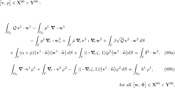
where
Remark 5.2 (The Brinkman equation). Notice that in the equation (89a), the product
 has been replaced by v2 · w2 (for consistency
 was replaced by f2 · w2). This is done in order to attain a Brinkman-type form in the third, fourth and fifth summands of equation (89a). Also notice that although
 and
and
 the product
 can not be replaced by
 due to the differential operators (the orthogonal matrix U depends on
 ). This is the reason why we give up expressing the activity on the interface Γ exclusively in terms of tangential vectors, as its is natural to look for.
5.3. Strong convergence of the solutions
In contrast to the asymptotic analysis in [14], the strong convergence of the solutions can not be concluded. The main reason is the presence of the higher order term x, weak limit of the sequence
 As it can be seen in the proof of Theorem 4.3, the higher order term x can be removed because the quantifier w2 belongs to Xtg. However, when testing the problem (30) on the diagonal [vє
, p
є] and adding the equations to get rid of the mixed terms, the quantifier v2,є does not belong to Xtg. As a consequence, the terms
As it can be seen in the proof of Theorem 4.3, the higher order term x can be removed because the quantifier w2 belongs to Xtg. However, when testing the problem (30) on the diagonal [vє
, p
є] and adding the equations to get rid of the mixed terms, the quantifier v2,є does not belong to Xtg. As a consequence, the terms
 contain in its internal structure inner products of the type

which can not be combined/balanced with other terms present in the evaluation of the diagonal. The product above is not guaranteed to pass to the limit
 because both factors are known to converge weakly, but none has been proved to converge strongly. Such convergence would be ideal since v2 ∈ Xtg, therefore
 and the term (90) would converge to zero. The latter would yield the strong convergence of the norms for
 and
and
 and the desired strong convergence would follow.
More specifically, the surface geometry states that the normal
 and the tangential directions (tg) are the important ones, around which the information should be arranged. On the other hand, the estimates yield its information in terms of
 (T) and z (N). Such disagreement has the effect of keeping intertwined the higher order and lower order terms to the extent of allowing to conclude weak, but not strong convergence statements.
5.4. Ratio of velocities
The relationship of the velocity in the tangential direction with respect to the velocity in the normal direction is very high and tends to infinity as expected for most of the cases. We know that
 is bounded, therefore
 Suppose first that
 and consider the ratios

The lower bound holds true for є > 0 small enough and adequate δ > 0; then we conclude that the L2-norms' ratio of the tangent component over the normal component blows-up to infinity, i.e., the tangential velocity is much faster than the normal one in the thin channel.
In contrast, if
 nothing can be concluded, since it can not be claimed that
 on Γ unless f2 = 0 is enforced, trivializing the activity on Ω2. Therefore, it can only be concluded that
 for є > 0 small enough, when
as discussed above.
for є > 0 small enough, when
as discussed above.
5.5. Reduction to the flat horizontal case
In this section we show how the e-problems (30) and the limit problem (77) are corresponding generalizations of the systems (23) and (59) presented in [14]. We show this fact in several steps:
a. Recall that in [14] the interface r is flat horizontal and, for convenience, it was assumed that Γ ⊂ ℝN-1 x {0}. In our current scenario, this is attained by merely setting ζ = 0, which satisfies all the conditions of Hypothesis 1. Furthermore, the following differential operators verify

where D є w is defined in (15).
b. For ζ = 0, the stream line localizer of Definition 2.5 is the constant matrix valued function
 where I ∈ ℝNxN is the identity matrix. In particular
 which is independent from

c. Given that the stream line localizer is the identity matrix, the normal and tangential velocities introduced in the equations (19) satisfy

Taking into account all the previous observations, the e-problems (30) reduce to
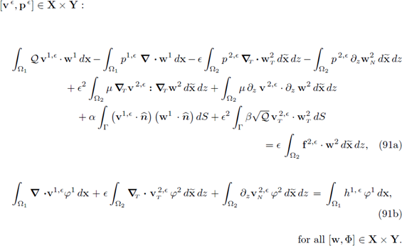
The summands of the second line in (91a) can be written in the following way:
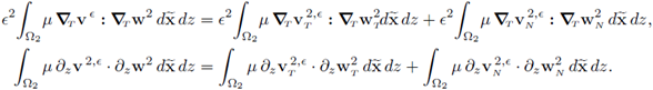
Introducing the changes above in (91), the system (23) in [14] is attained.
Again, taking into account the simplifications corresponding to a flat horizontal interface (ζ = 0) listed at the beginning of this section, the limit problem (77) reduces to
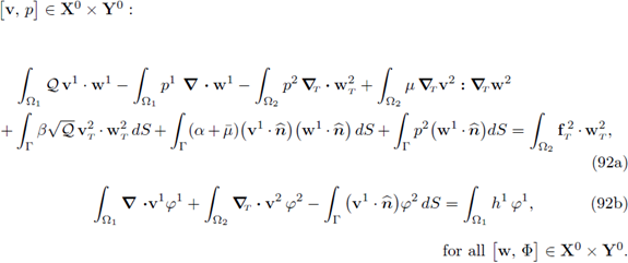
Notice that since ζ = 0, the spaces X00, Y00 in [14] are isomorphic to X0 and Y0 in (92), respectively. Finally, reordering the summands in the equalities above and writing
we obtain the system (59) in [14].
The є-problems (30) are isomorphic to the problems (23) in [14], and the limit problem (77) is isomorphic to (59) (Theorem 21) in [14]. In addition, the reasoning proving that (77) is the limit form of (30) stands for the case ζ = 0. Next, the strong convergence limitations discussed in Section 5.3 no longer hold, since the expression (90) reduces to

From here, the same reasoning presented in Section 5 in [14] applies.
The previous observations, show that the present work entirely recovers the weak convergence results analogous to those presented in [14], but extending them to a considerable broader scenario. On the other hand, the strong convergence properties in [14] could not be generalized, and they should be treated on a case-wise basis, using particular features of the function Z, as it was done in the equality (93) above.


