1. Introduction

Let G be a simple undirected graph with vertex set V (G) and edge set E(G). The degree of a vertex v ∈ V (G) is d(v) or simply dv. We denote by N(G) the number of vertices of the graph G. A graph G is bipartite if there exists a partitioning of V (G) into disjoint, nonempty sets V1 and V2 such that the end vertices of each edge in G are in distinct sets V1, V2. In this case V1, V2 are referred as a bipartition of G. A graph G is a complete bipartite graph if G is bipartite with bipartition V1 and V2, where each vertex in V1 is connected to all the vertices in V2. If G is a complete bipartite graph and N(V1) = p and N(V2) = q, the graph G is written as Kp,q. The Laplacian matrix of G is the n × n matrix L(G) = D(G) − A(G), where A(G) and D(G) are the matrices adjacency and diagonal of vertex degrees of G (⁷), (⁸), and (¹²), respectively. It is well known that L(G) is a positive semi-definite matrix and that (0,e) is an eigenpair of L(G) where e is the all ones vector. The matrix Q(G) = A(G)+D(G) is called the signless Laplacian matrix of G (see (⁴), (⁵), and (⁶). The eigenvalues of A(G), L(G) and Q(G) are called the eigenvalues, Laplacian eigenvalues and signless Laplacian eigenvalues of G, respectively. The matrices Q(G) and L(G) are positive semidefinite, (see (²¹)). The spectra of L(G) and Q(G) coincide if and only if G is a bipartite graph, (see (²), (⁴), (⁷), and (⁸)). The largest eigenvalue µ1 of L(G) is the Laplacian index of G, the largest eigenvalue q1(G) of Q(G) is known as the signless Laplacian index of G and the largest eigenvalue λ1(G) of A(G) is the adjacency index or index of G (³).

In (¹³), it was proposed to study the family of matrices Aα(G) defined for any real number α ∈ [0,1] as

Since A0(G) = A(G) and 2A1/2(G) = Q(G), the matrices Aα(G) can underpin a unified theory of A(G) and Q(G). In this paper, the eigenvalues of the matrices Aα(G) are called the α-eigenvalues of G. We write ρα(G) for the spectral radii of the matrices Aα(G) and are called the α-indices of G. The α-eigenvalue set of G is called α-spectrum of G. The spectrum of a matrix M will be denoted by Sp(M).

Let [l] denote the set {1,2,...l}. Given a rooted graph, define the level of a vertex to be equal to its distance to the root vertex increased by one. A generalized Bethe tree is a rooted tree in which vertices at the same level have the same degree. Throughout this paper {Bi : i ∈ [l]} is a set of generalized Bethe trees. Let Pl be a path of l vertices. In this paper, we study the tree Pl{Bi : i ∈ [l]} obtained from Pl and B1,B2,...,Bl, by identifying the root vertex of Bi with the i-th vertex of Pl where each Bi has order greater than or equal to 2. For brevity, we write Pl(Bi) instead of Pl{Bi : i ∈ [l]}. Let

In a graph, a vertex of degree at least 2 is called an internal vertex, a vertex of degree 1 is a pendant vertex and any vertex adjacent to a pendant vertex is a quasi-pendant vertex. We recall that a caterpillar is a tree in which the removal of all pendant vertices and incident edges results in a path. We define a complete caterpillar as a caterpillar in which each internal vertex is a quasi-pendant vertex.

A complete caterpillar Pl(K1,pi) is a graph obtained from the path Pl and the stars K1,p1,...,K1,pl by identifying the root of K1,pi with the i-th vertex of Pl where pi ≥ 1 for all i ∈ [l] (see Fig. 1 for an example). Let q ∈ [l]. Let Aq be the complete caterpillar Pl(K1,pi), where pq = n − 2l + 1 and pi = 1 for all i 6≠q.

Let Tn,d be the class of all trees on n vertices and diameter d. Let Pm be a path on m vertices and K1,p be a star on p + 1 vertices.

In (²⁰) the authors prove that the tree in Tn,d having the largest index is the caterpillar Pd,n−d obtained from Pd+1 on the vertices 1,2,...,d+1 and the star K1,n−d−1 identifying the root of K1,n−d−1 with the vertex [ d+1 2 ] .of Pd+1 In (¹⁰), for 3 ≤ d ≤ n − 4, the first [ d 2 +1] indices of trees in Tn,d are determined. In (⁹), for 3 ≤ d ≤ n−3, the first Laplacian spectral radii of trees in Tn,d are characterized. In (¹⁵) the authors present some extremal results about the spectral radius ρα(G) of Aα(G) that generalize previous results about ρ0(G) and ρ1/2(G). In (²⁴), the authors gives three edge graft transformations on Aαspectral radius. As applications, we determine the unique graph with maximum Aαspectral radius among all connected graphs with diameter d, and determine the unique graph with minimum Aα-spectral radius among all connected graphs with given clique number. In (¹⁴) the authors gives several results about the Aα-matrices of trees. In particular, it is shown that if T∆ is a tree of maximal degree ∆, then the spectral radius of Aα(T∆) satisfies the tight inequality

The complete caterpillars were initially studied in (¹⁸) and (¹⁹). In particular, in (¹⁸) the authors determine the unique complete caterpillars that minimize and maximize the algebraic connectivity (second smallest Laplacian eigenvalue) among all complete caterpillars on n vertices and diameter m + 1. Below we summarize the result corresponding to the caterpillar attaining the largest algebraic connectivity.

Theorem 1.1 (¹⁸) Theorems 3.3 and 3.6.). Among all caterpillars on n vertices and diameter m + 1, the largest algebraic connectivity is attained by the Caterpillar .

Theorem 1.2 (Abreu, Lenes, Rojo (¹)). Let α = 0,1/2. Let G be a complete caterpillars on n vertices and diameter m + 1. Then,

with equality if, and only if, .

Numerical experiments suggest us that is also the tree attaining the largest αindex in the class . In this paper we prove that this conjecture is true; we come up with a bound for the whole family Aα(G), which implies the result of Abreu, Lenes, and Rojo. This is organized as follows. In Section 2, we introduce trees obtained of the path Pl and the trees B1,B2,...,Bl by identifying the root vertex of Bi with the i-th vertex of Pl and give a reduction procedure for calculating their α-spectra, thereby extending the main results of (¹⁶). In the Section 3, we determine the graph that maximize the α-index in . We finish the section maximizing the α-index among all the unicyclic connected graphs on n vertices.

2. The α-eigenvalues of Pl(Bi)

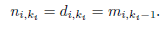
Given a generalized Bethe tree Bi with ki levels and an integer j ∈ [ki], we write ni,ki−j+1 for the number of vertices at level j and di,ki−j+1 for their degree. In particular, di,1 = 1 and ni,ki = 1. Further, for any j ∈ [ki − 1], let mi,j = ni,j/ni,j+1. Then, for any j ∈ [ki − 2], we see that

and, in particular,

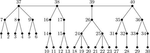
For i ∈ [l], it is worth pointing out that mi,1,...,mi,ki−1 are always positive integers, and that ni,1 ≥ ni,2 ≥ ··· ≥ ni,ki. We label the vertices of Pl(Bi) as in (¹⁶). (See figure 2).

Recall that the Kronecker product C ⊗ E of two matrices C = (ci,j) and E = (ei,j) of sizes m × m and n × n, is an mn × mn matrix defined as C ⊗ E = (ci,jE). Two basic properties of C ⊗ E are the identities

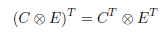
and

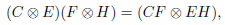
which hold for any matrices of appropriate sizes.

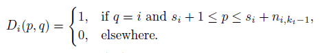
We write Il for the identity matrix of order l and jl for the column l-vector of ones. For be the matrix of order si × l defined by

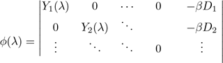
Let β = 1−α, and assume that Pl(Bi) is a tree labeled as described above. It is not hard to see that the matrix Aα(Pl(Bi)) can be represented as a symmetric block tridiagonal matrix

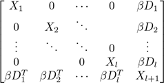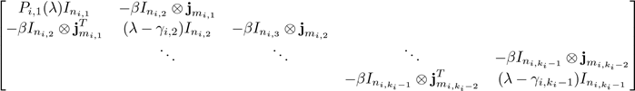
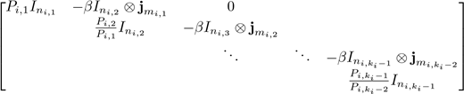
where, for i ∈ [l], the matrix Xi is the block tridiagonal matrix:

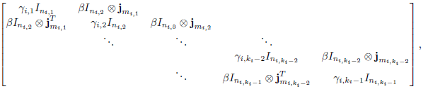and

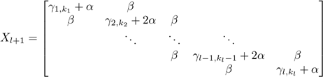where

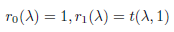
Let’s define the polynomials P0(λ),P1(λ),...,Pl(λ) and Pi,j(λ) for i ∈ [l] and j ∈ [ki] as follows:

Definition 2.1. For i ∈ [l] and j ∈ [ki], let

For i ∈ [l], let

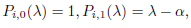
and for i ∈ [l] and j = 2,3,...,ki − 1, let

Moreover, let

and

For i = 2, 3,..., l - 1.

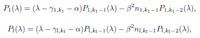
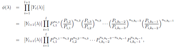
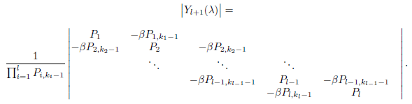
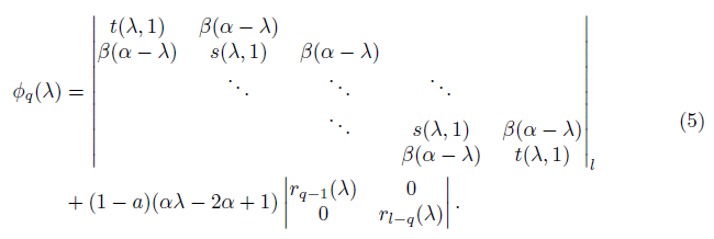
Theorem 2.2. The characteristic polynomial ϕ(λ) of Aα (Pl(Bi)) satisfies

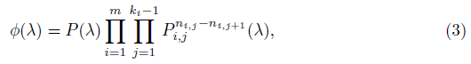
where

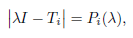
Proof. Write |A| for the determinant of a square matrix A. To prove 3, we shall reduce ϕ(λ) = | λI - Aα(pi)(Bi))|to the determinant of an upper triangular matrix. For a start,

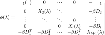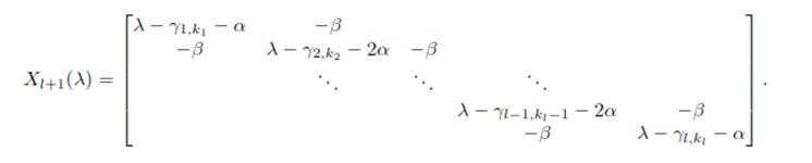
where, for i ∈ [l], the matrix Xi(λ) given by,

and

Let λ ∈ ℝ be such that Pi,j (λ) = ≠ 0 for any i ∈ [l] and j ∈ [ki −1]; set Pi, j = Pi, j (λ). For each i ∈ [l] and for all j ∈ [ki − 2], multiplying the j-th row of Xi(λ) inserted in ϕ( λ) by 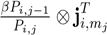and add it to the next row. Since

we obtain,

where, for i ∈ [l], the matrix Y_i(λ) is given by

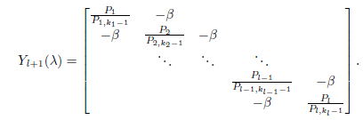
Thus, the equality (3) is proved whenever P_{i, j}(λ) ≠ 0 for any i ∈ [l] and j ∈ [k_i − 1]. Since for any i ∈ [l] and j ∈ [ki − 1] the polynomials P_i,j(λ) have finitely many roots, the equality (3) is verified for infinitely many value of λ. The proof is complete.

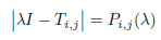
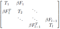
Definition 2.3. For i ∈ [l] and j ∈ [k _i −1], let T _i,j be the j×j leading principal submatrix of the k _i × k _i symmetric tridiagonal matrix

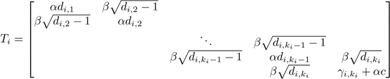
where β = 1 − α, c = 2 for i ∈ [l − 1] and c = 1 for i = 1 and i = l.

Since d _s > 1 for all s = 2,...,j, each matrix T _j has nonzero codiagonal entries and it is known that its eigenvalues are simple. Using the well known three-term recursion formula for the characteristic polynomials of the leading principal submatrices of a symmetric tridiagonal matrix and the formulas (1) and (2), one can easily prove the following assertion:

Lemma 2.4. Let α ∈ [0,1). Then

and

For any i ∈ [l] and j [ki - 1].

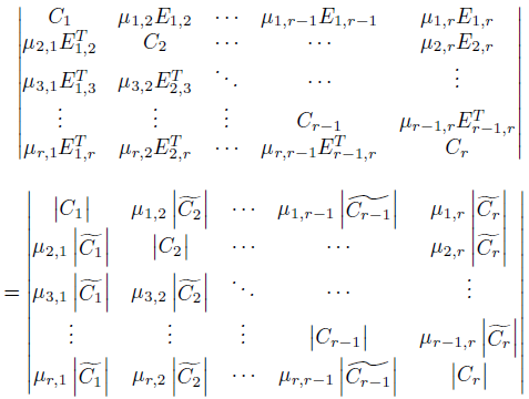
Let e à be the matrix obtained from a matrix A by deleting its last row and last column. Moreover, for i, j ∈ [r], let E_{i, j} be the k _i × k _j matrix with E _{i, j} (ki, k _j ) = 1 and zeroes elsewhere. We recall the following Lemma.

Lemma 2.5 (¹⁷). For i, j ∈ [r], let C _i be a matrix of order k _i x k _i and µ _{i, j} be arbitrary scalars. Then,

From now on, for −1], by F _i whose entries are 0, except for the entry F _i (k _i ,k _i+1 ) = 1.

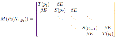
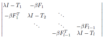
Lemma 2.6. Let 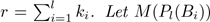be the symmetric matrix of order n × n

defined by

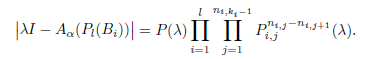
Then,

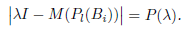
Proof. The characteristic polynomial of the matrix M (P _l (B _i )) is given by

From Lemma 2.5, we have that |λI - M (P _l (B _j ))| is given by

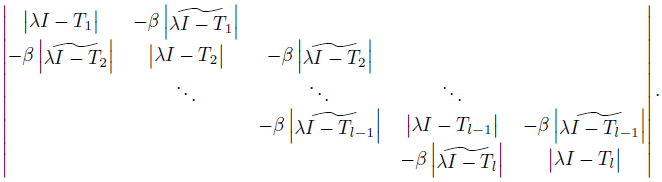
Since 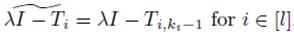, by Lemma 2.4, the proof is complete.

Theorem 2.2, Lemma 2.4, Lemma 2.6, and the interlacing property for the eigenvalues of hermitian matrices yield the following summary statement:

Theorem 2.7. Let α ∈ [0,1). Then:

3. The α-index of graphs

In Theorem 2.7, we characterize the α-eigenvalues of the trees P _l (B _i ) obtained from path P _l and the generalized Bethe trees B ₁ ,B ₂ ,...,B _l obtained identifying the root vertex of B _i with the i-th vertex of P _l . This is the case for the caterpillars P _l (K _1,pi ) in which the path is P _l and each star K _1,pi is a generalized Bethe tree of 2 levels. From Theorem 2.7, we get

Lemma 3.1. Let α ∈ [0,1). Then:

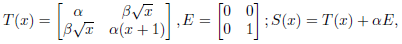
1. the α-spectrum of P _l (K _1,pi ) is formed by α with multiplicity and the eigenvalues of the 2l × 2l irreducible nonnegative matrix

where

2. ρ _α (P _l (K _1,pi )) is the largest eigenvalue of M(P _l (K _1,pi ));

3. ρ _α (P _l (K _1,pi )) > α.

Let t(λ,x) and s(λ,x) be the characteristic polynomials of the matrices T(x) and S(x), respectively. That is,

and

Then,

The notation |A| _t will be used to denote the determinant of the matrix A of order l × l. The next result is an immediate consequence of the Lemma 2.5.

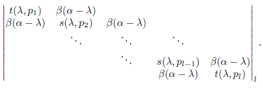
Lemma 3.2. The characteristic polynomial of M(P_l(K_1,pi )) is.

For q ∈ [l], let A _q be the complete caterpillar P _l (K _1,pi ) where p _q = n− 21 + 1 and p_{i = 1}for all i ≠ q. We define

and, for , we define

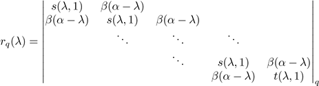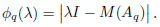
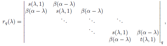
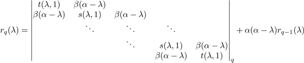
Let ϕ _q (λ) be the characteristic polynomial of M (A _q ), then,

Lemma 3.3. Let α ∈ [0, 1). Then

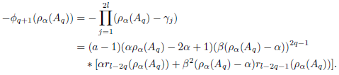
ϕ _q (λ)− ϕ _q+1 (λ) = (a−1)(αλ−2α+1)(β(λ−α)) ^2q−1 [αr _m−2q (λ)+β ²(λ−α)r _l−2q−1 (λ)] for all q ∈ [[ l+1 2 ]−1], where l ≥ 3.

Proof. By Lemma 3.2, the (q, q)-entry of ϕ _q (λ)= | λI - M(A _q )| is t(λ, α) if q =1 and s(λ, α) if q ≠ 1. . Let E _l ≌ P _l (K _1,pi ) where p _i = 1 for all i ∈ [l]. Let φ_s(λ)=| λI - M(E _S )|. From Lemma 3.2, we have

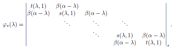
Since

and

For q= 2,…[ 𝑙 + 1 2 ]; then, expanding along the first row, we obtain

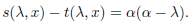
Since s(λ,x) = t(λ,x) + α(α − λ), by linearity on the first column, we have

Then,

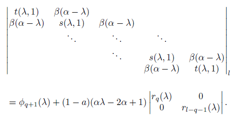
Let q ∈ - 1]. We search for the difference ϕ_q (λ) - ϕ_q+1(λ) We recall that (q,q)-entry of ϕ_q(λ) =|λI -M(Aq)| is t(λ, a) if q = 1 and s(λ, a) if q ≠1. Since t(λ,a) = t(λ,1) + (1 − a)(αλ − 2α + 1) and s(λ,a) = s(λ,1) + (1 − a)(αλ − 2α + 1), by linearity on the q-th column, we have

The (q + 1, q + 1)-entry of the determinant of order l on the second right hand of (5) is s(λ,1), and since s(λ,1) = s(λ,a) + (a − 1)(λα − 2α + 1), by linearity on the (q + 1)-th column, we obtain

Thereby,

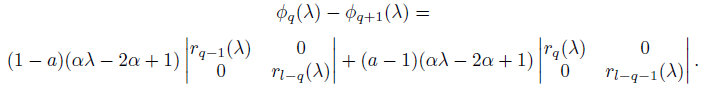
Thus,

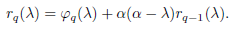
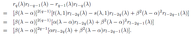
Applying the recurrence formula (4) to r _q (λ) and r _l−q (λ), we obtain

By repeated applications of this process, we conclude that

Hence,

Thus,

Let ρ(A) be the spectral radius of the square matrix A. From Perron-Frobenius’s Theory for nonnegative matrices ²³, if A is a nonnegative irreducible matrix then A has a unique eigenvalue equal to its spectral radius and it increases whenever any entry of it increases. Hence, we have the next result.

Lemma 3.4 (²²). If A is a nonnegative irreducible matrix and B is any principal submatrix of A, then ρ(B) < ρ(A).

Let C _n,l be the class of all complete caterpillars on n vertices and diameter l + 1. A special subclass of C _n,l is A _n,l = {A₁,A₂,...,A _l }, where A _q ^≌ P _l (K _1,pi ) ∈ C _n,l , with p _i = 1 for i ≠ q and p _q = n−2l+1. Since A _q and A _l−q+1 are isomorphic caterpillars for all q ∈ the next theorem gives a total ordering in A _n,l by the α-index.

Theorem 3.5. Let α ∈ [0,1). Then

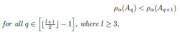
Proof. Let l ≥ 3. Let q ∈ . Let ϕ_q(λ) and ϕ_{q +1}(λ) be the characteristic polynomials of degrees 2l of the matrices M(A _q ) and M(A _q+1 ), respectively. The matrices M(A _q ) and M(A _q+1 ) are nonnegative irreducible matrices, then its spectral radii are simple eigenvalues.

Let

and

be the eigenvalues of the matrices M(A _q ) and M(A _q+1 ), respectively.

By Lemma 3.3, we have

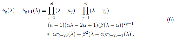
We recall that r_{l - 2q}(λ) and r_{l - 2q -1} (λ) are the characteristic polynomials of the matrices and whose spectral radii are and re-spectively. The matrices and are principal submatrices of M(A _q ). By Lemma 3.4, and Hence, r _l−2q (ρ _α (A _q )) > 0 and r _l−2q−1 (ρ _α (A _q )) > 0. We claim that ρ _α (A _q ) < ρ _α (A _q+1 ). Suppose ρ _α (A _q ) ≥ ρ _α (A _q+1 ). Then ρ _α (A _q ) ≥ γ _j for all j. Taking λ = ρ _α (A _q ) in (6), we obtain

By Lemma 3.1, ρ _α (A _q ) > α. Then αρ _α (A _q ) − 2α + 1 > 0. Thus,

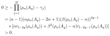
which is a contradiction. The proof is complete.^X

Lemma 3.6 (¹¹). Let A be a nonnegative symmetric matrix and x be a unit vector of ℝ ⁿ . If ρ(A) = x ^T Ax, then Ax = ρ(A)x.

Let N _G (v) be the vertex set adjacent to v in G.

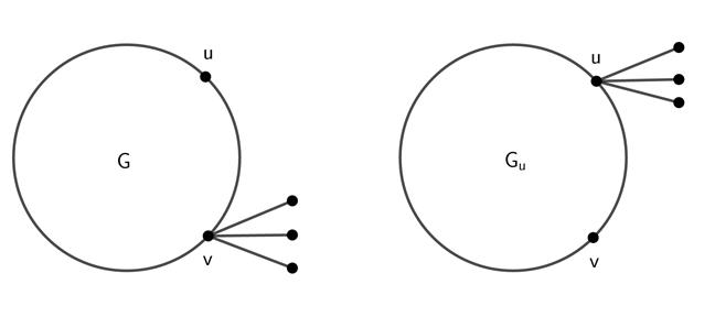
Lemma 3.7 (²⁴). Let α ∈ [0,1). Let G be a connected graph and ρ _α (G) be the αindex of G. Let u,v be two vertices of G. Suppose v ₁ ,v ₂ ,...,v _s , are some vertices of N _G (v) − (N _G (u) ∪ {u}) and x = (x ₁ ,x ₂ ,...,x _n ) is the Perron’s vector of A _α (G), where x _i corresponds to the vertex v _i for i ∈ [s]. Let

(as shown in Fig. 3). If x _u ≥ x _v , then ρ _α (G) < ρ _α (G _u ).

An immediate consequence of Lemma 3.7 is

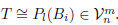
Theorem 3.8. Let T ∈ Then

Where . For α ∈ [0,1), the bound (7) is attained if, and only if, T ≌ . For α = 1, the bound (7) is attained if, and only if, T ≌A _k , where k = and , where m = 2.

Proof. Let α ∈ [0,1). Let Let x₁,x₂,...,x _l be the vertices of the path P _l in the tree T. Let B _i be a tree with k _i levels for all i ∈ [l]. Suppose T has the largest α-index in

Suppose k _i > 2 for some 2 ≤ i ≤ l − 1. Let u₁,...,u _si be all the vertices in the second level of B _i ; we can assume without loss of generality that u _si is an internal vertex. Let w₁,...,w _ri be all the vertices of N _G (u _si ) − {x _i }. Let

and

By Lemma 3.7, Moreover, and , which is a contradiction. If i = 1 or i = l, we reason analogously. Then, k _i = 2 for all i ∈ [l]. This is,

By reasoning analogously we can verify that

Let m ≥ 3. By Theorem 3.5,

Then the largest α-index is attained by For m = 2 the result is immediate. Let α = 1; then A _α = D, where D is the diagonal matrix of vertex degrees. Let . Let m = 3; then the maximum degree of T is less than or equal to n − 2l + 3. Then, ρ _α (T) ≤ n−2l+3 ≤ ρ _α (A _k ) for all k =2,…, [ 𝑚+1 2 ]. For m = 2 is result is immediate.