


 English (pdf)
 Article in xml format
 Article references
 Send this article by e-mail
 Cited by SciELO
  Cited by Google
  Similars in
SciELO
Similars in
SciELO  Similars in Google
 Permalink
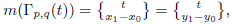
In the theory of smooth surfaces the Gaussian curvature plays a fundamental role as a tool to measure how these objects bend in Euclidean space. It is an intrinsic function depending only on distances that are measured on the surface, but not on how the surface is isometrically embedded in ℝ3. This result is the famous Gauss’ Theorema Egregium.
Can we detect this curvature by counting paths and measuring their length in a given surface? To fix ideas, let us consider a connected surface S and two given points p,q ∈ S. We will not consider all possible paths on S from p to q, but only simple ones as we shall explain. To settle down the problem, we start with the simplest case, i.e., the Euclidean plane R2, of constant curvature equal to zero, when equipped with Cartesian coordinates (x,y) and the Riemannian metric dx 2 +dy 2. The idea relies on looking only at paths built with straight lines parallel to the axes, and only moving forward. In other words, we concatenate a finite number of pieces of the flows ((x,y),s) 7→ (x + s,y), ((x,y),s) →7 (x,y + s), corresponding to the orthogonal vector fields ∂ x and ∂ y coming from the given coordinates. Then we can reach q = (x 1 ,y 1) from p = (x 0 ,y 0) if, and only if, x 1 ≥ x 0, y 1 ≥ y 0 and the time we need to do this is given by t = x 1 −x 0 +y 1 −y 0. In this way we have established the set Γ p,q (t) of all admissible paths. The first question is: how can we count or give a measure to this set? In this particular case, every element of Γ p,q (t) has the same length, i.e., t. Thus, independently of how we define the measure value m(Γ p,q (t)), when we add all these lengths, the result will be t · m(Γ p,q (t)). The conclusion is the following: in curvature zero the “sum” of all these lengths is equal to the average of the lengths of the external paths times the “number” of paths. The external paths are the one from (x 0 ,y 0) to (x 1 ,y 0) and then to (x 1 ,y 1), and the other from (x 0 ,y 0) to (x 0 ,y 1) and then to (x 1 ,y 1).
The aim of this note is to show that we can effectively define m(Γ p,q (t)) and the “sum”, or better, the integral of the length over Γ p,q (t), to prove that the phenomenon explained in the previous paragraph only occurs in the case of surfaces of curvature zero. We will transfer the situation of the Euclidean plane to S by using a local parameterization Ψ : U ⊆ R2 → S containing p = Ψ(x 0 ,y 0) and q = Ψ(x 1 ,y 1). Our calculations work for metrics of the form

where h, f: ℝ → ℝ are strictly increasing smooth functions. We remark that, when |f′′′ (s)| < h′(s), surfaces of revolution realize these spaces (see Section 4 for details). Since the classical surfaces of constant curvature, i.e, the plane ℝ2, the sphere S 2 and the Poincaré half plane H = ℝ >0 ×ℝ, can be realized locally as open revolution surfaces in ℝ3, our result is valid for these surfaces as well.
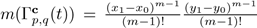
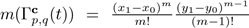
We will see that a good definition for the measure of the set of paths Γ
p,q
(t) explained above is given by
 where
where
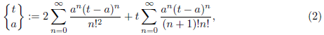
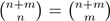
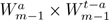
denotes the so called continuous binomial coefficient defined in 4. The name and suggestive notation come from the analogy with the binomial coefficient
 which counts the paths in the lattice N2 ⊂ ℝ2, from (0,0) to (m,n) ∈ ℕ2. Then, our main result is an explicit formula for the integral of the length associated to the Riemannian metric (1), which is the content of
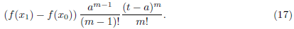
Theorem 1.1. The integral of the length over all admissible paths Γ p,q (t) from p = Ψ(x 0 , y 0) to q = Ψ(x 1 , y 1) in time t > 0 is given by
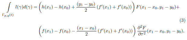
where t = x
1 − x
0 + y
1 − y
0 and
 . In particular, the integral is given by the measure of Γ
p,q
(t) times the average of the length of the external paths if, and only if, f is a quadratic function. For the surfaces of constant curvature, this happens only if the curvature is zero.
. In particular, the integral is given by the measure of Γ
p,q
(t) times the average of the length of the external paths if, and only if, f is a quadratic function. For the surfaces of constant curvature, this happens only if the curvature is zero.
This formula gives us a new insight on how the curvature of a surface affects the length of paths defined over it. We will prove it by studying a quite simple definition of a path integral and looking at the geometric information it contains.
It is worth remarking that several approaches to path integrals exist in the literature. The most famous ones are Feynman and Wiener integrals. Feynman integrals, although not fully formalized from a mathematical point of view, are used in Quantum Mechanics to capture physical information, (see 5), (6). The Wiener integrals are defined on sets of continuous paths in Euclidean space and model Brownian motion. However, the differential paths have Wiener measure zero, (see, e.g., [5, Theorem 1.1]), and hence do not have a notion of length. It could be interesting to see if the integral of length makes some sense in any of the mathematical formulations of Feynman integrals.
2. Paths as simplexes and their measure
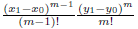
Coming back to the case of the plane R2, a path in Γ p,q (t) is determined, first, by the order in which we glue a finite number of segments given by the flows of ∂ x and ∂ y , and second, by the length of these segments: for the horizontal (resp. vertical) part, the length is x 1 − x 0, (resp., y 1 − y 0). Such order can be represented by a finite sequence c of the numbers 1 and 2, where 1 represents an horizontal segment and 2 represents a vertical one, i.e., by an element of the set

In this way, we can write
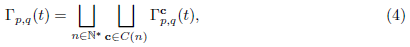
as a disjoint union, where each
 denotes the set of paths built with order c. If c ∈ C(n), a path γ ∈
corresponds to a vector s
denotes the set of paths built with order c. If c ∈ C(n), a path γ ∈
corresponds to a vector s
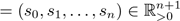 , where s
j
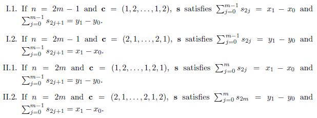
is the length of the jth segment of γ. We can distinguish four cases:
, where s
j
is the length of the jth segment of γ. We can distinguish four cases:
In all cases,
is given, up to a permutation of the variables, by the Cartesian product of two simplexes. Thus we can reduce the problem to measure usual simplexes in Euclidean space.
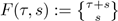
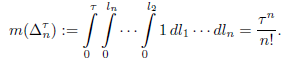
Given τ ≥ 0, we denote by

the n-symplex generated by the canonical vectors of ℝ n+1 , multiplied by τ. We can parameterize it by using

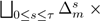
restricted to W n τ : = {(l 1 ,...,l n ) ∈ ℝ n |0 ≤ l 1 ≤ ··· ≤ l n ≤ τ}. The way we measure ∆ n τ is by calculating the n-volume of W n τ , i.e., by declaring that
If n = 0, we interpret this value as 1. Note that the variables involved are related by the formulas

By using the parameterization
 , we find that
 ,
,
formula that can be interpreted as a multiplicative counting principle in our setting. Moreover, if we fix
 can be written as the disjoint union
 . The measure we have introduced is compatible with this decomposition in the following sense:

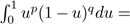
Note we have used here the elementary formula for the Beta function
 .
.
In this order of ideas, we have that
 for the cases I.1 and I.2,
 for the case II.1, and
for the case II.2. Finally, the measure of Γ p,q (t) is defined as the sum of the measures of its parts,
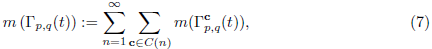
in agreement with the definition of the binomial coefficient
 given in the Introduction.
Remark 2.1. Our approach to associate this measure is based on the work 3. There the authors work more generally with a manifold M and a finite number of vector fields X
1
,...,X
k
defined over it. In this framework, if p,q ∈ M and t > 0 are given, the set of admissible paths Γ
p,q
(t) consists of piece-wise smooth paths from p to q formed by concatenations of the flows φ
j
of the X
j
using a total time t. Here there is also a decomposition of Γ
p,q
(t) analogous to (4), and if c = (c
0
.c
1
,...,c
n
) is a given order,
 can be embedded in
 .
.
3. On the continuous binomial coefficients
The motivation to introduce the power series
 , which converges for every t,a ∈ ℂ, came from measure or “count” elements of Γ
p,q
(t), thus we regard it as a continuous analogue (not extension) of the classical binomial coefficients. For extensions to complex variables, it is enough to write the usual binomial coefficients in terms of the Gamma function. For a more detailed study of this extension to real variables, see, e.g. 7.
, which converges for every t,a ∈ ℂ, came from measure or “count” elements of Γ
p,q
(t), thus we regard it as a continuous analogue (not extension) of the classical binomial coefficients. For extensions to complex variables, it is enough to write the usual binomial coefficients in terms of the Gamma function. For a more detailed study of this extension to real variables, see, e.g. 7.
To show the strong parallel with the discrete binomial coefficients, we highlight the following two properties:
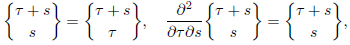
which corresponds to the discrete versions
 and
and
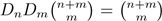 , respectively, and D
n
f = f(n+1)−f(n) is a difference operator. There are more analogies, for instance, continuous versions of Chu-Vandermonde’s formula, (see 8).
, respectively, and D
n
f = f(n+1)−f(n) is a difference operator. There are more analogies, for instance, continuous versions of Chu-Vandermonde’s formula, (see 8).
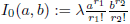
To perform some calculations we will need later, we can use the Bessel-Clifford function of the first kind (2, p. 358) which are defined by the power series
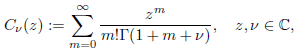
and where Γ denotes the classical gamma function. From the very definition, we note that
 and also

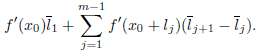
We can use the functions C 0 and C 1 to write

and also the remaining C n to write the derivatives

These equations are easily proved by using induction on n. For later use we need the following two formulas:
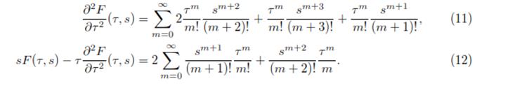
To prove (11), simply use (10) for n = 2, and (8) for v= 1 to obtain
 =
=

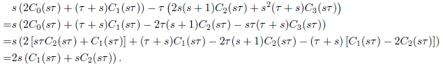
 In the same way, we use (8) for v = 0 and v = 1; so, see that the left-hand side of (12) is in fact
Remark 3.1. Bessel-Clifford functions are not so widely used since they can be written in terms the well-known modified Bessel functions I
ν
by means of the equation
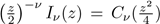 , (see [2, p. 375]). This formula can help us to determine the growth of the continuous binomial coefficients: from the asymptotic expansion of I
ν
(z) for fixed ν and large values of z [2, p. 377], we find that
, (see [2, p. 375]). This formula can help us to determine the growth of the continuous binomial coefficients: from the asymptotic expansion of I
ν
(z) for fixed ν and large values of z [2, p. 377], we find that
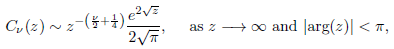
where the powers of z assume their principal value (here f(z) ∼ g(z) means that lim z→∞ f(z) / g(z) = 1 in the corresponding domain). Then, it follows from equation (9) that

4. Adding all the lengths
When working with the Riemannian metric (1), we find that the paths ϕ 1(s) = Ψ(x 0 + s, y 0) and ϕ 2(s) = Ψ(x 0 , y 0 + s), 0 ≤ s ≤ s 0, have lengths

respectively. Regarding the Gaussian curvature, it only depends on the x-coordinate and it is given by the formula
 , which can be easily checked by direct computations.
Our main example consists of surfaces of revolution. To fix ideas, consider an injective smooth curve η: (a,b) → ℝ3, η(s) = (α(s),0,β(s)) with α(s) > 0. When we rotate it around the z-axis, the map Ψ(s,ϕ) = (α (s) cosϕ, α (s)sinϕ, β(s)), (s, ϕ) ∈ (a, b)×(0, 2π) provides a parameterization, and the associated metric is given by
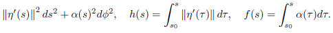
Note that if η is parameterized by arc-length, then h(s) = s − s 0. These surfaces realice the Riemannian metric (1) when |f′′(s)| < h′(s) because in this case we can simply take
α(s) = f′(s) and

If we choose h(s) = s and f(s) = −cos(s), 0 < s < π, the previous conditions are fulfilled and we obtain a typical local parameterization of the sphere S 2. On the other hand, by taking h(y) = f(y) = ln(y), the metric would be y−2 (dx 2 + dy 2), which is the metric of the Poincaré plane ℍ. Thus, if we put

and we change 1/s = sin(t), we recover the usual parameterization of the pseudosphere obtained by rotating the tractrix

This is a model of an open surface of constant Gaussian curvature equal to −1 (see, e.g., 1, p. 198]).
Naturally, if h(s) = f(s) = 1 we obtain the cylinder, which has curvature identically zero. Yet another model for curvature zero is the punctured plane in polar coordinates, i.e., η(s) = (s,0,0), s > 0, h(s) = s,f(s) = s 2 /2, and the metric ds 2 + s 2 dϕ 2. In these cases Theorem 1.1 shows that the integral of the length is given by the measure of Γ p,q (t) times the average of the lengths of the paths with configurations (1,2) and (2,1), since f is quadratic.
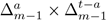
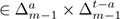
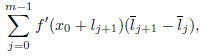
We are now in position to define and compute the integral of the length over Γ p,q (t), and thus to prove Theorem 1.1. The first observation is that the length of the horizontal part of any path in Γ p,q (t) is actually constant, and it is given by h(x 1) − h(x 0). Then, it is enough to calculate the integral of the length of the vertical parts. For this, we use the decomposition (4) and distinguish the four cases I.1, I.2, II.1 and II.2 as explained in Section 2. To simplify notations we will write a = x 1 − x 0 and t − a = y 1 − y 0.
Let us start with the case I.1, where Γ
p,q
c (t) is identified with
 , and thus we use the variables
 By using the second formula in (13), we see that the length of the vertical parts of a path corresponding to s
 is given by

When we integrate this function over
 , we find that it is given by

where I m− 1( a,t − a) is equal to
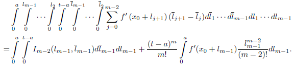
To solve this recurrence and the ones that will appear in the other cases, we can use the following
Lema 4.1. Let f: ℝ → ℝ be a differentiable function, and consider r,r
1
,r
2 ∈ ℕ, λ,x
0 ∈ ℝ, and a,b ∈ ℝ ≥ 0. If we define
 and
and
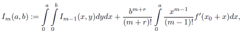
then

Proof. For m = 1 the formula is clear, so we assume it is valid for some m ∈ ℕ∗. Using the definition and the induction hypothesis we see that
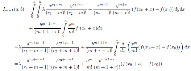
The result follows from the principle of induction.
By taking λ = 0, I 0 = 0, and r = 1 in Lemma 4.1, we find that (14) becomes

Note that any term with negative exponent is interpreted to be zero.
We proceed now with case I.2, where Γ
p,q
c (t) is again
 . In the variables
 the length of the vertical parts of a path is given by
The integral of this function over
 can be found as before by solving the same recurrence. Therefore, it is given by

For the case II.1,
 corresponds to
 and we work with the variables

The length of the vertical parts of a path in this case is
and the recurrence needed to calculate the integral of this function over
 is the same as in case (I.1), but with r = 0. Thus, we get
Finally, for the case II.2,
 corresponds to
 , the variables are
 ,
,
 and the length of the vertical
parts is given by
The recurrence here for the integral of the last sum over
 the same as
in case (I.1), but with r = 2. Thus, the integral is given by

Now, we define
 , the integral of the length over Γ
p,q
(t), as the sum of the integrals of the length of each of its part. For the horizontal parts, the result is
, the integral of the length over Γ
p,q
(t), as the sum of the integrals of the length of each of its part. For the horizontal parts, the result is
 , being this length the constant h(x
1) − h(x
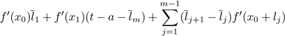
0). For the vertical parts, we add together (15), (16), (17) and (18) to get
, being this length the constant h(x
1) − h(x
0). For the vertical parts, we add together (15), (16), (17) and (18) to get
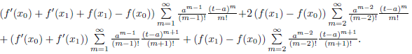
Then, by grouping common factors and taking into account formulas (11) and (12), the previous term is equal to

This proves formula (3) in Theorem 1.1. Finally, for the last statement of the theorem, note that it is equivalent to show that f satisfies the differential equation
whose solutions are precisely quadratic functions.


