


 Inglês (pdf)
 Artigo em XML
 Referências do artigo
 Enviar este artigo por email
 Citado por SciELO
  Citado por Google
  Similares em
SciELO
Similares em
SciELO  Similares em Google
 Permalink
1. Introduction
The mathematical perspective helps us to know the impact that public health strategies have on communities through the construction of mathematical models. Public health strategies are designed either to control or to eradicate an infectious disease, and these strategies are applied to certain groups. For example, treatment and isolation strategies target infectious individuals, and the vaccination strategy is applied to susceptible individuals. In other cases, public health strategies target certain core groups, for example, sexually active individuals can receive sexual education. It is known that each one of these strategies has a different impact upon the dynamics of the infectious disease when these are applied into the population. There are mathematical epidemiological models which analyze the behavior of the population if a public health strategy is being applied. For example, using differential equations, it has been analyzed how a disease treatment impacts a population whose individuals have gotten an infectious disease as measles, tuberculosis, or flu [6, 10, 17, 16, 18, 19]; also, Gumel et al. [7] and Eastwood et al. [5] analyzed the dynamics of SARS and H1N1 when infectious individuals are isolated or quarantined, respectively. In the same direction, Arino et al. [1] analyzed how applying a vaccine to a susceptible population affects the dynamics of infectious disease, and Hadeler and Castillo-Chavez [8] analyzed the influence of educational programs in the dynamics of an infectious disease.
In all cases mentioned above, a unique public health strategy was applied to control the spread of infectious diseases however, the study of combinations of public health strategies has been left sidestepped, even though, sometimes, two public health strategies are simultaneously applied to control a disease. For example, the only way to prevent measles is to get the measles, mumps, and rubella (MMR) vaccine, and infected patients should be isolated for 4 days in an airborne infection isolation room (AIIR). Sometimes, when a public health strategy is being applied by the State, for example, isolation of infectious individuals, susceptible individuals use the strategy of social distancing because they believe that the risk of infection will decrease with this control intervention.
Isolation of infectious individuals is a good procedure to smother the epidemic curve because the number of possible encounters of susceptible individuals with infectious individuals is reduced. That is, with this intervention control, the transmission rate of the disease is reduced. This public health strategy has been applied to control the outbreak of infectious diseases as cholera, diphtheria, ebola, Lassa fever, leprosy, measles, mumps, plague, smallpox, tuberculosis, typhus, and yellow fever [9]. On the other hand, speaking about the treatment of a curable infectious disease, it is common to assume that all the cases can be treated. So, when a treatment is applied into a population, the transmission rate of the disease is reduced because the infectious period is reduced, and the number of infectious individuals circulating decreases.
It was mentioned above that the application of a public health strategy may change the evolution of an infectious disease, but these changes are very difficult to quantify. In this sense, mathematical epidemiology is very useful if one wants to know how public health strategies may affect some epidemiological parameters. The most famous epidemiology parameter is the basic reproduction number, which is denoted by R 0 . The definition of R 0 is as follows: R 0 is the average number of secondary infections produced by a single infectious individual during its infectious period when it is introduced into a completely susceptible population [2].
It is known that mathematical epidemiological models with isolation may show not only the existence of a forward bifurcation in R 0 = 1 but also the existence of a Hopf bifurcation if some conditions over the parameters are satisfied [9]. Meanwhile, mathematical epidemiological models with treatment show the existence of a backward bifurcation in Ro = 1. In some cases, the model shows a bistability phenomenon if some conditions over the values of the parameters are satisfied see [3, 13, 16, 17, 18]; however, the existence of both phenomena have been little studied when they exist simultaneously. Figure 1 shows the cases mentioned above.
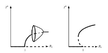
Figure 1 Case A) shows a forward bifurcation in Ro = 1 and a Hopf bifurcation when Ro > 1 while case B) shows a backward bifurcation in Ro = 1 and a bistability phenomenon for values of Ro < 1.
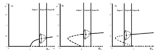
Figure 2 Case A) shows a forward bifurcation in R0 = 1 and a Hopf bifurcation when R0 > 1. Case B) shows a backward bifurcation in R 0 = 1 and a Hopf bifurcation for values of R 0 > 1 . Finally, case C) shows a backward bifurcation in R 0 = 1 and a Hopf bifurcation for values of Ro < 1 . Observe that, in the last case, a bistability phenomenon appears when R 0 < 1 .
The principal purpose of this paper is to show that both a periodic solution and a backward bifurcation can simultaneously occur for values of Ro less than 1. For this, two public health strategies will be simultaneously applied into a population. In particular, isolation and treatment of infected individuals.
In Section 2, an SIQR model with treatment is constructed, and the existence of the equilibrium points is analyzed. In Section 3, the direction of the bifurcation in R 0 = 1 for the proposed model is determined. We give conditions over the parameters of the model for which the model shows a Hopf bifurcation. In Section 4, numerical simulations of the solutions of the model are provided. Finally, in Section 5, we discuss the main results of the model analysis.
2. The model, equilibrium points, and R 0
Let N(t) be the total population, which is divided into: susceptible, infectious, isolated, and recovered individuals. Each class is denoted by S(t), I(t), Q(t) and R(t) respectively. Then N(t) = S(t) +1(t) + Q(t) + R(t). In epidemiological models, new infectious individuals are commonly modeled by 3NS, which is called standard incidence; Because we assume that some proportion of infectious individuals is isolated, this term must be replaced by the term
 . Notice that the fraction
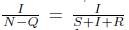 describes the infectious fraction of the circulating population. Also, we assume that some proportion of infectious individuals is treated to recover them. That is, a second public health strategy is simultaneously applied to the population. In epidemiological models, treated individuals are commonly modeled by the term αI. This term describes a scenario when the number of treated individuals may be so big as the number of infectious individuals, which is an unrealistic scenario. In this work, the treatment term is going to be replaced by the term
 , which is a bounded function. This term describes a treatment regime that is constrained either by the available budget or by the amount of human or material resources.
The epidemiological model with quarantine and treatment is
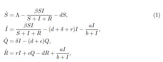
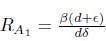
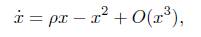
where the parameters of the model are defined as follows: β is the infectious rate of the disease, A is the recruitment rate of susceptible individuals, d is the per capita death rate, δ is the isolation rate, r is the natural recovery rate of the disease, e is the removal rate of Q class, and
 is the treatment rate, which is a decreasing function of the infectious individuals.
 describes how the public health system loses attention capacity as a function of the infectious individuals. Observe that, a is the maximum value of the recovery rate.
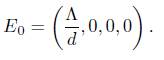
The disease-free equilibrium for model (1), which exists for all values of the parameters, is given by
The Jacobian matrix associated to model (1) is shown here
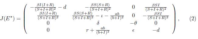
where i = d + δ + r and θ = d + Є.
A first result about the behavior of the model solutions of (1), at the beginning of the epidemic outbreak, is showed as follows.
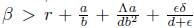
Theorem 2.1. Let
 The disease-free equilibrium of model (1) is locally asymptotically stable if, and only if, Ro < 1.
Proof. The eigenvalues associated to the Jacobian matrix (2) evaluated in E 0 are
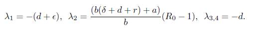
Then, all the eigenvalues are negative real numbers if, and only if, R 0 is less than 1. Therefore, the result is proved.
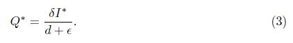
Endemic equilibrium points for model (1) can be obtained by setting the left-hand side of each differential equation equal to zero. Then, solving the third one, the equilibrium value for the quarantined individual is obtained, and it is given by
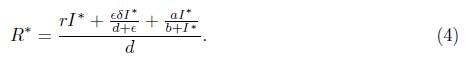
Substituting Q * into the fourth equation of model (1), the equilibrium value for the recovered individuals R * is given by
The number of susceptible individuals in the equilibrium is
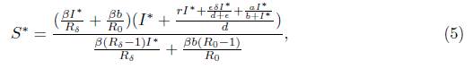
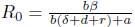
which is obtained when the expression for Q* and R* are replaced in the first equilibrium condition of model (1). Notice that,
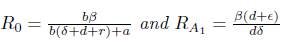
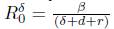 is the basic reproductive number for the SIQR model without treatment [9].
When analyzing R0, we note that e does not affect R
0
and R
δ
0
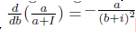
because e is not related to the infectious process. Also,
 ; in contrast,
 . Then, by increasing either the parameter 6 or a, R
0
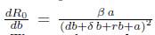
decreases. That is, the number of secondary infections decreases as a function of a number of isolated or treated individuals. On the other hand, by increasing b, R
0
increases since by increasing b the velocity in which infectious individuals are treated at the beginning of the epidemic is decreasing as a function of the parameter b. In other words,
. Then, by increasing either the parameter 6 or a, R
0
decreases. That is, the number of secondary infections decreases as a function of a number of isolated or treated individuals. On the other hand, by increasing b, R
0
increases since by increasing b the velocity in which infectious individuals are treated at the beginning of the epidemic is decreasing as a function of the parameter b. In other words,
Finally, substituting the equilibrium coordinates S*, Q*, and R* into the second equilibrium equation and simplifying the expression, the equilibrium equation, for I *, is obtained. This is a cubic equation which is given by I * f (I *) = 0, where
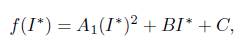
and the coefficients of the quadratic function, f (I*), are given by;
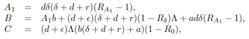
Where
 .
.
Analyzing the coefficients, it is observed that A i > 0 ⇔ Ra 1 > 1, and C < 0 R0 > 1.
By examining the quadratic function f( I * ) , the following result is achieved.
Theorem 2.2. For model (1) with
 .
.
1. When R 0 > 1 and Ra 1 > 1 or R 0 < 1 and Ra 1 < 1, there is exactly one endemic equilibrium.
2. When R 0 < 1 and Ra 1 > 1, there are exactly two endemic equilibria if B < 0 and B 2 - 4A i C > 0.
3. When Ro < 1 and Ra 1 > 1, there is one endemic equilibrium if B < 0 and B2 - 4AiC = 0. Otherwise there are none.
Each scenario shown above is important, but there is a relevant case where there is an equilibrium point that bifurcates into two equilibrium points. Such equilibrium solution satisfies that B2
- 4A
i
C = 0 when
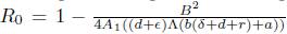 . This particular value of Ro is denoted by R
o
*
, and it is going to be fundamental in the bifurcation analysis of the equilibria solutions.
. This particular value of Ro is denoted by R
o
*
, and it is going to be fundamental in the bifurcation analysis of the equilibria solutions.
Notice that, R δ 0 > R 0 for all α > 0. Analyzing the expression (5), if R δ 0 < 1, then S* < 0.
3. Stability analysis
The centre manifolds theory allows a reduction of the dimension space where the system can be analyzed, and the theory of the normal forms grants to associate more simple differential equations to the system. The resulting differential equations are analyzed in a neighborhood of the equilibrium points and their dynamical behaviors are useful to understand the dynamics of the original system. For this purpose, for model (1), the direction of the bifurcation in R o = 1 will be analyzed [4, 12].
First, system (1) is translated to the origin using the changes of variables
 , y = I, z = Q, and w = R. Because the non-linearities of model (1) make it difficult to analyze the stability of the trivial solution of the model, the vector field associated to system (1) is analyzed using Taylor's series for each equation of the translated model. It allows to separate the linear and non-linear terms of the series as follows:
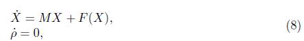
Where
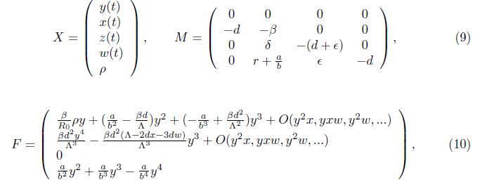
and p = R 0 - 1.
By using the eigenvectors associated with the linearization of model (1) in a neighborhood of R 0 = 1, the matrix T is constructed.
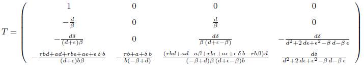
The matrix T transforms the Jacobian matrix M given by (3) into the (real) Jordan canonical form.
We calculate T -1 to transform system (1) into one simplified system
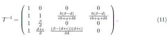
By using T -1 , an adequate variable change, and algebraic simplifications, we obtain the next differential equation on the centre manifold at the bifurcation point.
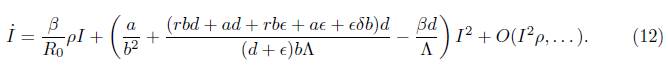
The dynamics of the model is analyzed only in the last equation because the centre manifolds acts as an attractor.
Notice that, equation (12) is associated with the normal form
which is the normal form by a transcritical bifurcation.
For the analysis, we consider the second order coefficient of the equation (12), which is given by
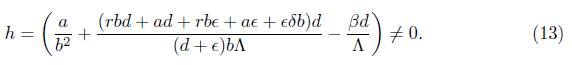
Then, a backward bifurcation is presented in model (1) when R
0
= 1 if, and only if,
 . Therefore, if a backward bifurcation appears, the branch of the equilibrium point for model (1) that is emerging from R
0
= 1 is given by unstable endemic equilibrium points.
. Therefore, if a backward bifurcation appears, the branch of the equilibrium point for model (1) that is emerging from R
0
= 1 is given by unstable endemic equilibrium points.
The dynamical behavior of the equilibrium points that are far from the disease-free equilibrium is unknown because we make a local analysis around R n = 1. To complete the dynamical portrait of the model solutions, the next theorem will be used to describe the stability of an endemic equilibrium that belongs to the branch of equilibrium points associated with the backward bifurcation, which is denoted by E*. We show that a Hopf bifurcation may occur around E*. In this case, both backward and Hopf bifurcation will be occurring simultaneously.
It is known that a Hopf bifurcation arises from an equilibrium point whose stability changes because of the crossing of a pair of complex conjugate eigenvalues over the imaginary axis. In other words, a Hopf bifurcation in E* exists if: first, the characteristic polynomial, which is associated to E0, has a pair of complex conjugate roots,
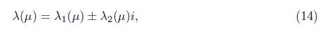
second, μ 0 is a critical value such that
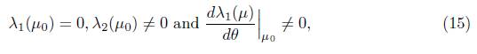
third, the remaining eigenvalues of the Jacobian matrix have non-zero real parts.
The first two Hopf conditions are very precise; however, calculating the eigenvalues associated with the differential equation system can be very difficult. Jing and Lin [11] and Sheng and Lin [15] provided criteria for the existence of a Hopf bifurcation. They proved that conditions (14) and (15) can be written in terms of the coefficients ci for i = 1,.., n of the characteristic equation

which is associated with a differential equation system.
To do this, they used the so-called Hurwitz matrix of which there are n and they are shown in the following.
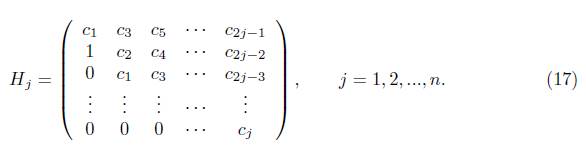
Now, we enunciate the Theorem 3 proved in [15].
Theorem 3. For (16), if the following conditions are satisfied
(i) μ = μ 0 is a zero of the Hurwitz determinantffn-1(μ) = 0,
(ii) H n -2 = 0,Hn-3(μ0 ) = 0,Cj (μ0 ) > 0, j = 1, ...,n,
(iii)
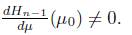
Then the conditions (14) and (15) of the existence of the Hopf bifurcation are satisfied.
The third condition is related to bifurcation points. So, we analyze where the equilibrium point E* changes its stability.
Theorem 3.1. Let E* be an endemic equilibrium point for system (1). For some conditions over the model parameters, a Hopf bifurcation occurs in E * . That is, a family of periodic solutions bifurcates from E * .
Proof. The Routh-Hurwitz criteria mention that the endemic equilibrium point E* is locally asymptotically stable if, and only if, both the coefficients c i of the characteristic polynomial and the Hurwitz determinants Hi that are associated with the model are positive, see [14].
By calculating the characteristic polynomial associated to the linearization of system (1) in E * , we obtain

Where
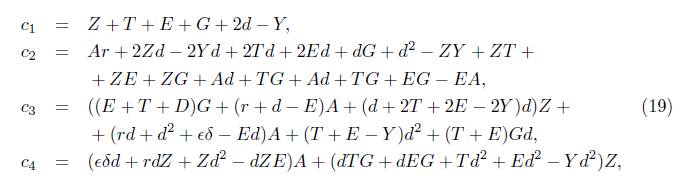
and


For the characteristic polynomial (18), the Hurwitz determinants are given by H 1 = c 1 , H 2 = c 1 c 2 - c3, H 3 = c 1 c 2 c 3 - c 1 2 c 4 - c 2 3 , and H 4 = c 4 H 3 . Notice that, any of the coefficients c i or the Hurwitz determinants H i may be negative. Then, in this case, the criteria are not satisfied, and the endemic equilibrium E* is unstable.
We will analyze numerically the Hopf conditions because the resulting expressions are algebraically intractable. Notice that, the determinants H i are functions of the parameters of model (1). We will use the Hurwitz determinants to seek a solution of the equation H n-1 (μ 0 ) = 0 which is the first condition of Theorem 3. This solution will be substituted into the other conditions of Theorem 3, and finally, we will verify that all conditions of the Theorem 3 are satisfied. In particular, with d = 0.000039, r = 0.07, δ = 0.4, e = 0.025, A = 2, α = 0.001249473466, β= 0.026 and 3 = 0.51 the three conditions are satisfied. In summary, there is a Hopf bifurcation for these values of the model parameters.
In the next section, numerical simulations will illustrate different scenarios for the model solutions. In particular, we show the existence of stable periodic orbits for values of the parameters inside the Hopf curve.
4. Numerical Simulations
Numerical simulations of the solutions of the model will be shown. For this, XPPAUT 7.0 is used. In particular, the bistability phenomenon is displayed when R 0 < 1. This bistability phenomenon is given either by a periodic orbit and the disease-free equilibrium or by an endemic equilibrium and the disease-free equilibrium.
The values of the parameters used in the last section correspond to the average life time
 = 70.25 years, the average infectious period of approximately
 , that is equivalent to 2 weeks, the period of
 days before an infectious the individual is isolated and the isolation period of
 days.
days.
First, we show a scenario, for model (1), with a backward bifurcation in R 0 = 1 without the bistability phenomenon. For this, scenario, ∧ = 2, α= 0.001249473466, β = 0.026 and 3 = 0.51. With these values of the parameters R 0 = 0.9843741757 and RO = 1.085016350.Figure 3 shows this scenario. Observe that, the typical behavior of the solutions when R 0 belongs to the region I of Figure 2 B) is that solutions go to the disease-free equilibrium.
In the second place, we show a scenario where a stable limit cycle exists for R 0 > 1 (see Figure 2 B), region II). In this case, the equilibrium point E* belongs to the branch of the endemic equilibrium points that arises from a backward bifurcation in R 0 = 1.Figure 4 shows the behavior of the infectious class for different values of the infection rate. In this case, we only vary β. β = 4, 5, 6.9,10, for which R 0 is 7.72, 9.65,13.32,19.30 and R δ is 8.5,10.64,14.68, 21.27, respectively.
Figure 3 The behavior of the solutions of model (1) with different initial conditions and R 0 * < R 0 < 1. In this case, two unstable endemic equilibria exist, which are saddle node points. Also, the disease-free equilibrium is locally asymptotically stable.
Once that a stable limit cycle exists, it can be destroyed when R 0 increases (see Figure 2 Region III). Figure 5 shows the stabilizing effect of the rate a over the oscillations of the solutions of model (1). In this example, β = 6.9 and α = 0.001, 0.0012, 0.00125. For these parameters values, R 0 = 13. 57, 13. 37, 13. 33, respectively. The value of the other model parameters is the same as the above case.
Figure 4 Existence of a limit cycle for model (1). The size of the period and the amplitude of the solution are reduced when (3 is increasing.
Figure 6 Backward bifurcation in R0 = 1 and Hopf bifurcation when R0 < 1. Case A) shows that the non-trivial equilibria solutions are unstable. In this case, the bistability phenomenon does not appear. In this case, the solutions go to the disease-free equilibrium. Case B) shows that the infectious disease persists in a periodic orbit. In this case, the bistability phenomenon appears. Case C) Ro < 1 shows the classical backward bifurcation. In this case, the endemic equilibrium is locally asymptotically stable.
Finally, we show a scenario with both a backward bifurcation in R 0 = 1 and a stable limit cycle when R 0 < 1; see Figure 6B). In this scenario, the bistability phenomenon occurs. For this example, the values of the parameters are given by β = 17, b = 0.026, S = δ, Є= 0.025, d = 0.8, r = 0.04, A = 2, α = 0.4528. For these values of the parameters R δ 0 = 0.70087 and R 0 = 2.485380117. In particular, Figure 6 shows how the values of α affects the stability of the endemic equilibrium in E*. In this case, we only vary α= 0.4535,0.4528, 0.4510. For these values of α, R 0 = 0.700098,0.70087,0.7028.
5. Discussion
Knowing the impact that public health strategies have on a population is a paramount objective in mathematical epidemiology. There are so many epidemic models that explore the behavior of the solutions when a unique public health strategy is used a control intervention; in contrast, in the mathematical epidemiology literature, there are very few epidemic models that explore the effect due to two different public health strategies acting simultaneously in a community.
The model analysis shows that the simultaneous application of two control interventions has a great impact on the evolution of the disease. In particular, it is easier to bring R 0 below 1 using both control strategies because R 0 decreases as a function of the number of isolated or treated individuals. However, the application of two strategies to decrease the number of infectious individuals does not preclude the possibility there exist multiple endemic equilibriums for R 0 < 1 and sustained oscillations in the number of infectious individuals for R 0 > 1 . In contrast, both phenomena can coexist for some values of the parameters of the model.
In particular, the simultaneous application of treatment and isolation of infectious individuals can show three plausible scenarios if a backward bifurcation exists. In the former case, the number of infectious individuals goes to the disease-free equilibrium for all initial conditions. This is the result expected by decision-makers. In the second case, the number of infectious individuals goes to the disease-free equilibrium or to the endemic equilibrium. This scenario is the classical bistability phenomenon. In this case, if the solutions of the model go to zero or nontrivial equilibrium depends on the initial conditions. Finally, depending on the initial conditions, the number of infectious individuals goes to the disease-free equilibrium or goes to one stable periodic solution. In particular, sustained oscillations can appear even though R 0 > 1. In this scenario, the Hopf bifurcation appears in the upper branch of the backward bifurcation. This periodic orbit can be destroyed for some values of the parameters.
In summary, the simultaneous application of treatment and isolation of infectious individuals can lead to catastrophic scenarios even though, intuitively, we think that applying two strategies are better than applying just one.

