


 English (pdf)
 Article in xml format
 Article references
 Send this article by e-mail
 Cited by SciELO
  Cited by Google
  Similars in
SciELO
Similars in
SciELO  Similars in Google
 Permalink
1. Introduction
The Nonlinear Complementarity Problem, (NCP), which in some contexts is synonymous with system in equilibrium, arises among others, in applications to Physics, Engineering, and Economics [3], [8], [14], [19]. The problem is to find a vector x Є ℝ n such that x ≥ 0, F(x) ≥ 0 and x T F(x) = 0, with F: ℝn → ℝn continuously differentiable. Here, a vector is nonnegative if all its components are nonnegative. A widely used technique for solving the NCP is to reformulate it as a system of nonlinear equations using a complementarity function φ: ℝ2 → R such that
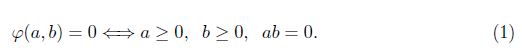
Then, we consider Ф: ℝ n - ℝ n and define the nonlinear system of equations
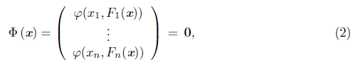
which is a nondifferentiable system due to the lack of smoothness of φ. From (1), a vector
x*
is a solution of (2), if, and only if,
x*
it is a solution of the NCP. To solve (2) and thus, to solve the NCP, a nonsmooth algorithms type Newton [27], [29] and quasi-Newton [20], [21], among others [1], [6], [22], [26], [31] have been proposed. The natural merit function [24] Ψ: ℝ
n
→ ℝ, defined by
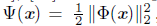 , is used in the globalization of these methods. Thus, Ψ(x) is minimized in ℝn. These methods use the concept of generalized Jacobian [10] defined by the set

for a Lipschitz continuous function G: ℝ n → ℝ n , in x, where D G denotes the set of all points where is G is differentiable and hull {A} is the convex envelope of A. This set is nonempty, convex, and compact [11]. Usually, the set (3) is difficult to compute, for this reason, we use the overestimation ∂G(x) T ⊆ ∂G 1 (x) x… x ∂G n (x) given in [11], where the right side, for short BeG(x) T [18], called C-sub differential of G at x, is the set of matrices ℝ nxn , whose i-th column is the generalized gradient of the i-th component of the function G.
Another strategy to solve (2) is to smooth the Jacobian proposed in [9] and called Jacobian smoothing in [18]. The general idea of methods using this strategy is to approximate Ф by a smooth function Ф μ : ℝ n → ℝ n , where μ > 0 is the smoothing parameter, and then solving a sequence of smooth nonlinear equation systems,
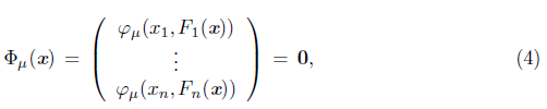
with μ going to zero and φ μ a smoothing function of φ used in (2). The system (4) is solved at each iteration by solving the mixed Newton equation) Ф’μ(xk)sk = - Ф (xk).
In [18], the authors present a new algorithm with good numerical performance based on the Jacobian smoothing strategy to solve the NCP, by reformulating it as a system of nonlinear equations using the Fischer-Burmeister complementary function defined by
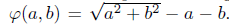 . Motivated by the results obtained with this function, and since it is a particular case of the following family of complementary functions [17]

corresponding to λ = 2, in this paper we use this strategy with the family (5) to propose a new algorithm that solves complementarity problems by reformulating it as a nonlinear, nondifferentiable system of equations. This algorithm can be seen as a generalization of the one proposed in [18] to any member of family φλ, with λ in (0, 4). Under certain hypotheses, we demonstrate that the proposed algorithm converges local and, q-superlinear or q-quadratically to a solution of the complementarity problem. In addition, we analyze the numerical performance of the proposed algorithm.
The organization of this paper is as follows. In Section 2, we present the Jacobian smoothing strategy applied to a function Фλ, we described the Jacobian matrix of its smoothing and find λ Section 3, we present some preliminary results that we use to develop the convergence theory of the algorithm proposed. In Section 4, we present a new Jacobian smoothing algorithm to solve nonlinear complementarity problems that generalize the one presented in [18] to all members of family (5). Moreover, we prove that our algorithm is well defined. In Section 5, we develop its global convergence theory. In Section 6, under some hypotheses, we prove that the algorithm converges local and q-superlinear or q-quadratically to the solution of the complementarity problem. In Section 8, we analyze the numerical performance of the proposed algorithm. Finally, In Section 9, we present our concluding remarks.
2. Smoothing Jacobian strategy for Фλ(x) = 0
We consider the reformulation (2) of the NCP as a nonsmooth nonlinear system of equations. If φ = φλ, the family (5), we obtain the system Фλ(x) = 0. The basic iteration of a generalized Newton method to solve this system has the form,

where H k Є ∂Фλ(x k ) or H k Є ∂ c Фλ(x k ). Here, we use H k Є ∂ c Фλ (x k ). In order to define a smoothing Jacobian method for Фλ (x) = 0, we follow the basic idea given in [18] and we consider smoothing φλ as proposed in [4]: for all λ Є (0,4) and μ > 0,

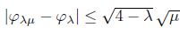
As expected, the distance between φλ and its smoothing function, φλμ, is upper bounded by a constant that depends on the parameters λ and μ. This is a particular case of the following proposition that will be useful in the convergence theory.
Proposition 2.1. Function φλμ satisfies the inequality

for all (a,b) Є ℝ2
and μ
1
,μ
2
μ 0. In particular,
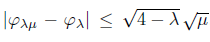 , for all (a,b) Є ℝ2, λ Є (0, 4) and μ ≥ 0.
Proof. Let (a, 6) Є ℝ 2, μ 1 and μ 2 nonnegatives, such that μ 1# μ 2.

Observe that
 . Then

In particular, if μ
1
= μ and μ
2
=0 then
 .
.
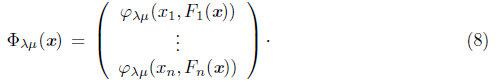
From (7), we define the function φλμ: ℝ n → ℝ n by,
The next proposition gives an upper bound for the distance between φλ and its approximation φλμ.
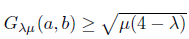
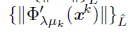
Proposition 2.2. The function φλμ satisfies the following inequalities
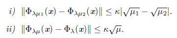
for all x Є ℝ n, and μ, μ
1
, μ
2 ≥ 0, where
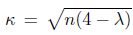 .
.
Proof. Using the Euclidean norm and Proposition 2.1,
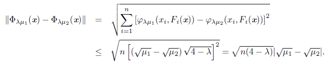
The second part of the proposition is obtained by choosing μ 1 = μ and μ 2 = 0.
Now, the basic iteration of a smoothing Jacobian method for solving φλ (x) = 0 is as follows
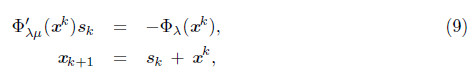
where Ф’ λμ (x k ) is the Jacobian matrix of Ф’ λμ at x k . From (6) and (9), we have that this method solves the reformulation Ф λ (x) = 0, replacing H k Є ∂ C Ф λ (x), with an approximation Ф ’λμK (x k ). Thus, these methods can be seen as quasi-Newton. The Jacobian matrix Ф ’λμ (x) is given by
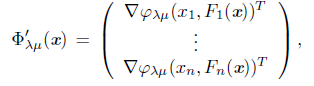
where
 , with

where
 .
.
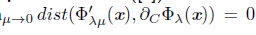
The next proposition guarantees that, if j tends to zero, the distance between Ф ’λμ (x) and ∂ C Ф λ (x) also tends to zero. Thus, it makes sense to replace the Newton iteration (6) with (9).
Proposition 2.3 ([4]). Let x Є ℝ
n
be arbitrary but fixed. Then we
 .
.
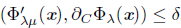
From this proposition, for every δ > 0 there exists 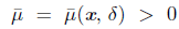 such that dist
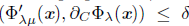 , for all
 . In our algorithmic proposal is very important to obtain an expression of J since it gives an upper bound of μ. For this, we proceed as in [18] and we obtain the following proposition.
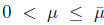
Proposition 2.4 ([30]). Let x Є ℝ n be arbitrary but fixed. Assume that x is not a solution of the NCP and define
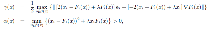
with β(x) = {i: xi = 0 = Fi(x)} . Let δ > 0 and define
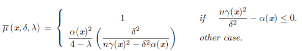
Then distp
 , for all μ such that
 .
.
Since our algorithmic proposal is a global algorithm for solving the NCP, indirectly through its reformulation Фλ(x) = 0, we consider the natural merit function Ψλ : ℝ n → ℝ defined by
 . The idea is to solve the NCP by minimizing
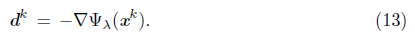
Ψλ. But, there is a problem: the direction computed from (9), is no necessarily a descent direction for Ψλ at xk. Following [18], an alternative is to use this direction to reduce the related merit function
3. Preliminaries
In this section, we present some definitions, propositions, and lemmas related to the nonlinear complementarity which will be useful in the development of the convergence theory of our algorithmic proposal.
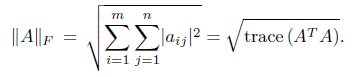
Definition 3.1. Let A Є ℝ nxn. The Frobenius norm of A is defined by
Definition 3.2. Let A Є ℝ nxn and M ⊆ ℝ nxn be a nonempty set of matrices. The distance between A and M is defined by, dist(A, M) = inf BeM {||A - B||}, where || • || is a matrix norm.
Definition 3.3. Let {tk} ⊆ ℝ, if there exists a number U such that
1. For every Є > 0 there exists an integer N such that k > N implies tk < U + Є.
2. Given Є > 0 and m > 0, there exists an integer k > m such that tk > U - Є.
Then U is called the superior limit of {tk} and we write U = limsuxpk →∞ tk.
Related with a solution x* of the NCP, we have the following index sets,

When β # 0, x* is called a degenerate solution.
Definition 3.4. Let x* be a solution of the NCP.
1. If all matrices in ∂ BФλ(x*) are nonsingular, x* is called a BD-regular solution.
2. If the submatrix 1 F'(x*)ââ is nonsingular and the Schur complement
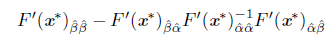
is a P-matrix2, x* is called an R-regular solution.
Definition 3.5. Given the sequences {αk} and {βk} such that βk ≥ 0, for all k, and αk = O(βk), if there exists a positive constant M such that |αk| ≤ Mβk, for all k. We write αk = o(βk), if αk/βk = 0..
Proposition 3.6 ([17], [28]). Assume that limk→∞ {xk} C ℝ n is a sequence converging to x*. Then,
1. The function Φλ is semismooth, so ||Φλ(xk)−Φλ(x∗)−Hk(xk−x∗) || = o(∥xk−x∗∥), for any Hk ∈ ∂CΦλ(xk).
2. If F is continuously differentiable with locally Lipchitz Jacobian then Φλ is strongly semismooth; that is, ||Φλ(xk) − Φλ(x∗) − Hk(xk − x∗)||= O(||xk − x∗||2), for any Hk ∈ ∂CΦλ(xk).
Proposition 3.7 ([18]). Given x Є ℝ n and μ> 0 arbitrary but fixed, then

Proposition 3.8 ([23]). If x* Є ℝ n is an isolated accumulation point 3 of a sequence {xk} ⊆ ℝ n such that q||xk+1 - xk ||} L converges to zero, for any subsequence {xk}L converging to x* . Then xk converges to x*.
Proposition 3.9 ([13]). Let G: ℝ n → ℝ n be locally Lipschitz and x* Є ℝ n such that G(x*) = 0, satisfary all matrices in ∂ G(x*) are nonsingular and assume that there exist two sequences {xk} ⊆ ℝ n and {dk} ⊆ ℝ n with

Then ||G(xk + dk)|| = o (||G(xk)||) .
Proposition 3.10 ([30]). Let x, z Є ℝ n such that ||x - z|| ≤ α ||x||, α Є (0,1). Then xT(x - z) ≤ α ||x||2.
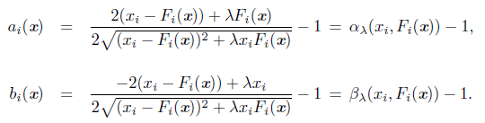
Proposition 3.11. [17] Let x Є ℝ n arbitrary. Then
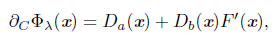
where Dα = diag(α1(x), .. ., α n(x)), Db = diag(b1(x),.. ., bn(x)) are diagonal matrices in ℝ nxn.
. If (xi,F(xi)) = (0, 0), then
■ If (xi,F(Xi)) = (0, 0) then αi(x) = σi - 1 and bi(x) = Pi - 1, for any (σi,pi) Є ℝ 2 such that
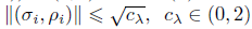 .
.
Proposition 3.12 ([17]). The merit function Ψλ is continuously differentiable and ∇ Ψλ(x) = V TΦλ(x), for any V ∈ ∂CΦλ(x).
Lemma 3.13 ([30]). Let μ > 0 and λ Є (0,4). The function h: (0, ∞) → ℝ, defined by is strictly decreasing.
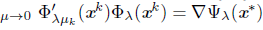
Lemma 3.14 ([30]). Let [xk} ⊆ ℝ n and {μk} ⊆ ℝ two sequences such that {xk} → x* for some x* Є ℝ n and {pk} → 0. Then limk→∞ ∇ Ψλ μk (xk) = ∇ Ψλ (x*) and lim
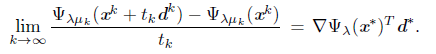
Lemma 3.15 ([18]). Let {xk}, {dk} ⊆ ℝ n and {tk} ⊆ ℝ with xk+1 = xk + tk dk such that xk → x*, dk → d* and {tk} → 0 for some vectors x*, d* Є ℝ n. Moreover, consider {μk} ⊆ ℝ a sequence such that {μk} - 0. Then
4. New algorithm
In this section, we propose a new algorithm for solving the NCP. Basically, the proposal is a generalization of the smoothing Jacobian method proposed in [18], and its basic iteration is given in (9). To guarantee the algorithm to be well-defined for an arbitrary NCP, we use a gradient step for Ψλ when linear system (11) solution does not exist or gives a poor descent direction for Ψλ μ.
Algorithm 1. (Smoothing Jacobian method),
SO.
 .
.
S1. If ||∇ Ψλ(xk)|| ≤ Є, stop.
S2. Find dk Є ℝ n solving the linear system of equations,
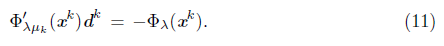
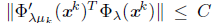
If the system (11) is not solvable or if the condition

is not satisfied, set
S3. Find the smallest mk Є {0,1, 2,...} such that

if dk is given by (11), and such that

if dk is given by (13). Set tk = θmk and xk+1 = xk + tk dk.
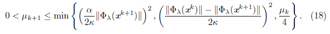
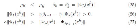
S4. If

set (βk+1 = ||Фλ(xk+1)|| and choose μk+1 such that,

If (16) is not satisfied and dk = -∇Фλ(xk) then set βk+1 = βk, and choose μk+1 such that
If none of the above conditions is met, set βk+1 = βk and μk+1 = μk.
S5. Set k = k + 1 and return to S1.
In SO, we introduce the parameters and initialize the variables. In S1, it is natural to think that the algorithm stops when the gradient of the merit function becomes too small. However, in the implementation, we add other classic criteria like maximum number of allowed iterations and one that prevents the algorithm from no finding an adequate step size. In S2, the calculus of a search direction is perhaps the main step of the algorithm: we find dk by mixed Newton equation (11). In case of (11) is not solvable or the direction does not satisfy descent criteria (12), we use the steepest descent direction of the merit function (13), which guarantees a descent direction of Ψλ.
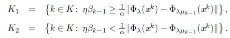
After finding the descent direction, the algorithm is globalized in step S3 using a line search which depends on this direction: if it is obtained by the Newton equation (11), the line search is made using (14), which is also used in [9] as a global strategy. On the other hand, if it is the steepest descent direction (13), the line search (15) is type Armijo [12]. The update of μk, in S4, starts with the condition (16) used in en [9]. If it is satisfied, μk is updated by (17). This guarantees that the distance between the subdifferential and smoothing Jacobian is small, and that μk tends to zero. If (16) is not satisfied, μk is updated by (18). The conditions (18) and (16) are essential to guarantee the algorithm to be well defined and to converge globally. For the convergence analysis of the algorithm, we define the following set

which is motivated by condition (16). Moreover, K = {0} U K1 U K2 (disjoint union), where
The next proposition is useful to demonstrate that the algorithm is well-defined. Its demonstration is analogous to that given in [18].
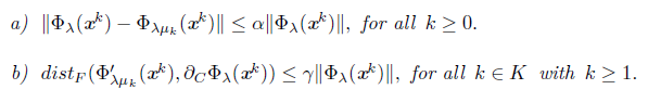
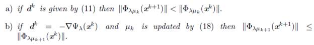
Proposition 4.1. The following inequalities hold:
The following result guarantees that Algorithm 1 is well-defined: it ends in a finite number of steps.
Proposition 4.2. Algorithm 1 is well-defined.
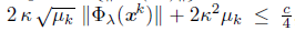
Proof. It is essentially the same given in [9]. It is sufficient to prove that mk in S3 is finite, for all k Є ℕ. In effect, if a descent direction is given by (13) then the condition Armijo-type guarantees that mk is finite [18]. On the other hand, let assume that the direction is given by (11). Since Ψλμk is continuously differentiable and its gradient is given by
 , by Taylor's Theorem, we have

Using the Newton's direction (11) in (20),
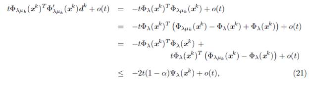
where the last inequality follows from Propositions 3.10 and 4.1. On the other hand,
Therefore, from (20), (21) and (22),
 . This allows to conclude that exists a nonnegative integer mk such that (14) is satisfied.
5. Global convergence
In this section, we present the convergence results of the algorithm proposed. Basically, we prove that any accumulation point of the sequence generated by Algorithm 1 is a stationary point of Ψλ. These results generalize those presented in [18] for an algorithm using the Fischer-Burmeister function, which in turn is based on the theory developed in [9] for smoothing Newton-type methods. The proofs of the theorems and lemmas in this section and in the next section use the same steps as the proofs of the corresponding theorems in [18].
We start with two lemmas whose proofs use the updating rules of Algorithm 1.
Lemma 5.1. Assume that a sequence generated by Algorithm 1 has an accumulation point x*, which is a solution of the NCP. Then the index set K defined by (19) is infinite and the sequence {μk} → 0.
Proof. Assume that K is finite. For the updating rule (16) there exists an integer k0, such that βk = βk0. Moreover, ||Фλ(xk+1) || > ηβk0, for all k ≥ k0, which contradicts that x∗ is a solution of the NCP.
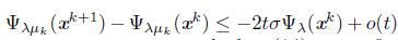
Lemma 5.2. The following statements hold:
Proof. Part a) is verified using the updating rule (14), and part b) is true if (16) is satisfied. In addition, we use Proposition 2.2 and some algebraic manipulations. 0
The next corollary is an important consequence of the previous result. Corollary 5.3. If
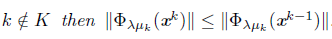 .
.
Proof. The proof is the same as Corollary 5.3 in [18].
The two following results are technical lemmas; they give some bounds that we use in the proof of Proposition 5.6. Details of the proofs are given in [30].
Lemma 5.4 ([30]). Assume that K is ordered like this k0=0 < k1 < k2 < .... Let k Є ℕ be arbitrary but fixed and kj the largest integer in K such that kj ≤ k then
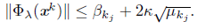
Lemma 5.5 ([30]). Assume that K is ordered like this ko =0 < k1 < k2 < .... Let k Є ℕ be arbitrary but fixed and kj the largest integer in K such that kj ≤ k. Then
 where
where
Using the two previous lemmas, we prove that the iterations xk stay at the same level set. This is important because we minimize different merit functions and a decrease in one does not imply a decrease in the other. This set can be arbitrary close to the level set Ψλ(x0).
Proposition 5.6. The sequence generated by Algorithm 1 stays in the level set
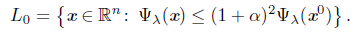
Proof. We assume, without loss of generality, that the set K given by (19) is ordered like this k0 = 0 < k1 < k2 < ..., which does not indicate that K is infinite. We consider k Є ℕ, arbitrary but fixed and kj the largest integer in K such that kj < k. From Lemmas 5.4 and 5.5, we have
 where r is defined by (23), that is.

Then
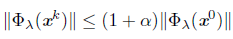 . Therefore, xk Є L0.
The following proposition is a consequence of inequality (24).
Proposition 5.7. Let {xk} be a sequence generated by Algorithm 1 and assume that the set K is infinite. Then each accumulation point of {xk} is a solution of the NCP.
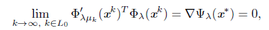
Proposition 5.8. Let {xk} be a sequence generated by Algorithm 1 and let {xk}L be a subsequence converging to
 for all k Є L, then x* is a stationary point of Ψλ.
Proof. If K is infinite, the accumulation point, x* is a solution of the NCP by Proposition 5.7. Thus, this is a global minimum and therefore, a stationary point of Ψλ.
If K is finite, we can assume that K ∩ L = 0 since the sequence has an infinite number of elements. Therefore, the updating rule (18) is satisfied for all k Є L, and consequently, the sequence {μk} converges to zero. Since K is finite there exists the largest element that we call k. Using the updating rules defined in step S4 of Algorithm 1, we have the following inequalities
Let assume by contradiction that x* is not a stationary point of Ψλ . That is, ∇Ψλ (x*) = 0. First, we prove that liminfkЄL tk = 0. For this, let assume liminf tk = t* > 0. Since dk = - ∇Ψλ (xk) for all k Є L, using Armijo-rule (15), we have that

for all k Є L sufficiently large, where c = σt* ||∇Ψλ (x*)||2 > 0. Since {μk} converges to zero, Proposition 2.2 guarantees that, for all k G N, sufficiently large,

Using again that {pk} converges to zero, the sequence {||Ф λ(xk)||} is bounded; since K is finite, we have, by Proposition 5.6, that
 , for all k Є ℕ, sufficiently large. If L = {l0,l1... } then, for all lj, sufficiently large, we have, in analogous way than in Proposition 5.6, that,
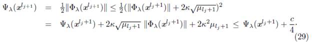
From (28) and (29),

 , for all lj, sufficiently large. Then the sequence
 as j → ∞, which contradicts that Ψλ(x) ≥ 0 for all x Є ℝ n. Therefore, liminfkЄL tk = 0.
If necessary, we can assume, from a subsequence, that limkЄL tk = 0. Hence, a full stepsize never is accepted for all k k Є L, sufficiently large. From Armijo-rule (15), we obtain
 or, equivalently,
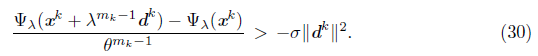
By taking the limit k → ∞ on L, we obtain from (30), the continuous differentiability of
 for all k Є L and the fact that θmk-1 → 0 for k → ∞, in L,

- This implies that σ ≥ 1, which is clearly a contradiction with the initial choice of parameter σ. Therefore,
The following lemmas are useful results for the proof of the main global convergence theorem.
Lemma 5.9. Let {xk} be a sequence generated by Algorithm 1 and let {xk}L be a subsequence converging to x* Є ℝn. If dk is a Newton direction for all k Є L, and the set K is finite, then the sequence {||dk||} is bounded, that is, there exist positive constants m and M such that

Proof. Let assume that dk is a Newton direction for all k G L, Thus, for these indices, we have that

If
 on a subset
 then, from (32),
 because
 is bounded on the convergent sequence
 . The continuity of Ф
λ
would imply that Ф
λ
(x*) = 0 and, from Lemma 5.1, K would be infinite, contradicting that K is finite. On the other hand, from (12), for all k Є L,
. The continuity of Ф
λ
would imply that Ф
λ
(x*) = 0 and, from Lemma 5.1, K would be infinite, contradicting that K is finite. On the other hand, from (12), for all k Є L,

Since
 is convergent (either by Lemma 3.14 or because μ
k
is constant, for k sufficiently large) and therefore bounded, there exists a positive constant C such that
is convergent (either by Lemma 3.14 or because μ
k
is constant, for k sufficiently large) and therefore bounded, there exists a positive constant C such that
 for all k Є L. From this and (33), we have
 for all k Є L. Since p> 1, {||d
k
||}
L
is bounded, which guarantees (31).
for all k Є L. Since p> 1, {||d
k
||}
L
is bounded, which guarantees (31).
Lemma 5.10 ([30]). Let {x k } be generated by Algorithm 1 and {x k } L a subsequence converging to x* Є ℝ n . If d k is a Newton direction for k Є L, and K is finite, then liminfkeL t k = 0.
Proof. The details of the proof are given in [30].
The next theorem is the main convergence result of the proposed algorithm.
Theorem 5.11. Let {x k } a sequence generated by Algorithm 1. Then each accumulation point of {x k } is a stationary point of .
Proof. If K is infinite, Proposition 5.7 guarantees the conclusion of this theorem. If K is finite and k denote its largest index then (25) to (27) are satisfied for all k ≥ k. On the other hand, let x* be an accumulation point of {x k }. There exists a subsequence {x k } L of {x k } converging to x*. If d k = - ∇Ψλ (x k ) for a finite number of index k Є L, Proposition 5.8 guarantees that x* is a stationary point of Ψ λ . Without loss of generality, we assume that d k is a Newton direction for all k Є L. Since K is finite, we can assume that for all k Є L, it is satisfied that k Є K, thus the updating rules (17) and (18) do not apply to these indices.
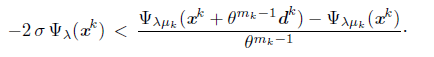
We proceed by contradiction and assume that x* is not a stationary point of the function Ψ λ .That is, Ψ λ (x*)=0. By Lemma 5.10, liminf kЄL t k = 0. Let L 0 be a subsequence of L such that {t k } L0 converges to zero. Then, m k > 0 for all k Є L 0 , sufficiently large, where m k Є ℕ is the exponent in (14). Then, -2σ θ mk-1 Ψ λ (x k ) < Ψ λμ k (x k + θ mk-1 d k ) - Ψ λμ k (x k ) for all k Є L 0 , sufficiently large. Dividing both inequalities by θ mk-1 , we obtain
Let μ* be the limit of {μ k } and if μ* = 0, we denote ∇ Ψ λμ* (x*) for the gradient of the unperturbed function Ψ λ in x . From (31), we can assume (through a subsequence) that {d k } L0 - d* =0. By taking the limit k - ∞, we obtain

For μ * = 0, this follows from Lemma 3.15. If μ * > 0, then μ k = μ * for k sufficiently large, then (34) follows from the Mean Value Theorem. Using (11), (27) and

Proposition 2.2, we have that, for all

 passing to the limit k - ∞, k Є L
0
, from (34) we obtain (and from Lemma 3.14, if μ * = 0 ),
passing to the limit k - ∞, k Є L
0
, from (34) we obtain (and from Lemma 3.14, if μ * = 0 ),

From Proposition 5.6, {Ψ
λ
(x
k
)} is bounded. Moreover,
 , since {μ
k
} converges. We have that Ψ
λ
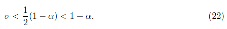
(x*) > 0, (in another case, K would be infinite). Therefore, from (35), σ ≥ (1 - a), which contradicts that σ < (1 - α). This completes the proof.
, since {μ
k
} converges. We have that Ψ
λ
(x*) > 0, (in another case, K would be infinite). Therefore, from (35), σ ≥ (1 - a), which contradicts that σ < (1 - α). This completes the proof.
6. Local convergence
In this section, we prove under certain hypotheses that the algorithm proposed converges locally and q-superlinearly or q-quadratically. The first result gives a sufficient condition for the convergence of a sequence x k generated by Algorithm 1.
Theorem 6.1. If one of the accumulation points of {x k } , let us say x*, is an isolated solution of the NCP, then {x k } converges to x*.
Proof. From Lemma 5.1, the index set K defined by (19) is infinite and {μ k } converges to zero. Therefore, Proposition 5.7 guarantees that each accumulation point of {x k } is also a solution of the NCP. Thus, x* must be an isolated point of {x k } . Let assume that x k L is an arbitrary subsequence of x k converging to x . Using the updating rule of S3 in Algorithm 1, we have

From (36), it is enough to prove that {d k } L → 0. We have that

because Ψ
λ
is continuous differentiable and the solution x* is a stationary point of 1
x
. If {d
k
}
L
has a finite number of Newton directions then it converges to zero. Because of this, let us assume that there exists a subsequence {d
k
}
L0
of {d
k
}
L
such that d
k
is a solution of (11) for all k Є L
0
. From (13),
 , for all k Є L
0
, thus,
, for all k Є L
0
, thus,

since p > 1. Since {x k } → x* and {μ k } - 0, with k Є L 0 , the Lemma 3.14 allows to conclude that,
and this implies that the right side of (38) converges to zero; therefore, {d k } L0 → 0. From (38), we have that {d k } L\L0 → 0, if L \ L 0 is infinite. Tims, Crom (36), we have that {||x k+1 - x k || }L → 0 , and therefore, from Proposition 3.8, {x k } converges to x*.
The two following results are technical lemmas that we will use in the proof of Theorem 6.6. The first one guarantees that, for all k Є K, the matrices Ф’ λμk (x k ) are nonsingular and its inverses are bounded. The second guarantees that the Newton direction satisfies the descent condition (12), for all k G K, with k sufficiently large. The details of the proof of each lemma are given in [30].
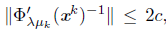
Lemma 6.2 ([30]). Let {x k } be a sequence generated by Algorithm 1. If one of the limit points, lets us say, x , is a R-regular solution of the NCP then for all k G K ; sufficiently large, the matrices Ф’ λμk (x k ) are nonsingular and its inverses satisfies that || Ф’ λμk (x k ) -1 || ≤ 2c, for some positive constant c.
Lemma 6.3 ([30]). Under the hypotheses of Lemma 6.2, the solution of linear system (11) satisfies the descent condition (12) for all k G K sufficiently large.
The following result will be useful to verify that Algorithm 1 eventually takes the full stepsize t k = 1. Its proof is the same of Lemma 3.2 en [9].
Lemma 6.4 ([30]). If there exists a scalar
 such that

 , for some k Є K and y Є ℝ n
, then
, for some k Є K and y Є ℝ n
, then
 , where μk is the smoothing parameter in the k-th step of Algorithm 1.
The next lemma guarantees that the indices of the iterations x k remain in K. By repeating this argument, we will guarantee that k Є K and t k = 1 for all k Є ℕ, suiciently large.
Lemma 6.5. Assume the hypotheses of Lemma 6.2. There exists an index k Є K such that for all k ≥ k, the index k + 1 also remain in K and x k+1 = x k + d k .
Proof. By Lemma 6.2, there is c > 0 such that
 , for all k Є K suiciently large. For this k, from the Algorithm 1, we have
Here,
 is such that dtst
F
is such that dtst
F
 Υβk, where the inequality is obtained by the part b) of the Proposition 4.1. Moreover, using Proposition 3.6 and since β
k
→ 0, we have
Υβk, where the inequality is obtained by the part b) of the Proposition 4.1. Moreover, using Proposition 3.6 and since β
k
→ 0, we have

with k → ∞ for k Є K. From this and Proposition 3.9 we have

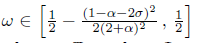
with k → ∞. for k Є K. Let
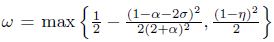 , where α, η and σ are the constants defined by Algorithm 1. From (41), there exists an index k Є K such that

for all k Є K with k ≥ k. Then, from Lemma 6.4,
 . Thus, full step is accepted for all k ≥ k, k Є K. In particular, x
k+1
= x
k
+ d
k
. From (42) and the definition o ω, we have
. Thus, full step is accepted for all k ≥ k, k Є K. In particular, x
k+1
= x
k
+ d
k
. From (42) and the definition o ω, we have
 which implies k + 1 Є K. By repeating this process, we can prove that, for all k ≥ k, itholds k Є K and x
k+1
= + d
k
.
which implies k + 1 Є K. By repeating this process, we can prove that, for all k ≥ k, itholds k Є K and x
k+1
= + d
k
.
The next result gives suicient conditions for the rate of convergence of Algorithm 1.
Theorem 6.6. Let {x k } be generated by Algorithm 1. If one of its limit points, let us say x*, is a R-regular solution of the NCP, then {x k } converges to x* at least q-superlinearly to x*. If F is continuous differentiable with Jacobian matrix locally Lipschitz, the convergence is q-quadratic.
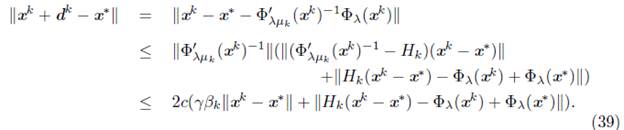
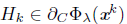
Proof. Lemma 6.5 guarantees that k Є K and t k = 1, for all k Є N sufficiently large. Then the q-superlinear convergence is obtained from (40). If F is continuous differentiable with Jacobian matrix locally Lipschitz, then by Proposition 3.6, we have ||H k (x k + d k ) -Ф λ (x k ) + Ф λ (x*) || = O(|| x k - x* || 2 ). Since Ф λ is locally Lipschitz, βk = || Ф λ (x k ) || = || Ф λ (x k ) - Ф λ (x*) || = O(|| x k - x* ||). Using these two inequalities in (39), ||x k + d k - x* || = O(|| x k - x* || 2 ); therefore, {x k } converges q-quadratically to x*.
7. Numerical results
In this section, we analyze the global numerical performance of Algorithm 1 and compare it with three global methods for solving the NCP. The first, a nonsmooth quasi-newton method proposed in [5] which we call Algorithm 2. The second, a smoothing Jacobian method proposed in [18] which, unlike our proposal, uses a smoothing of the Fischer function (Algorithm 1 with λ = 2), which Algorithm 3 and, the third, a smooth Newton method proposed recently in [32], which we call Algorithm 4. We vary λ in two forms obtaining two versions of our algorithm, namely, Method 1: we use the dynamic choice of λ used in [5], (this strategy combines the eiciency of Fisher function far from the solution with that of the minimum function near to it), Method 2: we vary randomly λ in the interval (0, 4). We finalized the section with a local analysis of our algorithmic proposal.
For the parameters, we use the following values: p = 10-18 , p = 2.1, θ = 0.5, σ = 10-4,Υ= 30, α= 0.95, η = 0.9, Є1= 10-12 Є2 = 10 -6 , k max = 300, t min = 10 -16 (minimum stepsize in linear search), where Є1 , Є 2 are the tolerances for Ф λ (x k ) and || ∇ Ψ λ (x k )||, respectively [18].
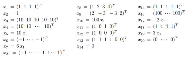
For the numerical test, we consider nine complementarity problems associated with the functions Kojima-Shindo (Koj-Shi), Kojima-Josephy (Koj-Jo), Mathiesen modificado (Math mod), Mathiesen (Mathiesen) Billups (Billups) [7], [25]; Nash-Cournot (Nash-Co) [16], Hock-Schittkowski (HH 66) [32], Geiger-Kanzow (Geiger-Kanzow) [15], Ahn (Ahn) [2]. We implemented Algorithms 1 (with Methods 1 and 2) and the test functions in MATLAB and use the following starting points taking from [5], [32],
To analyze the global convergence of Algorithm 1 and the variation of λ, we generate 100 random initial vectors for each problem with each of the methods described previously. We present the results in Table 1, which contains the problem and the method used to choose the parameter λ; the execution average time in seconds (t); the average number of iterations (k), and the percentage of times that the algorithm finds a solution to the problem (Success (%)).
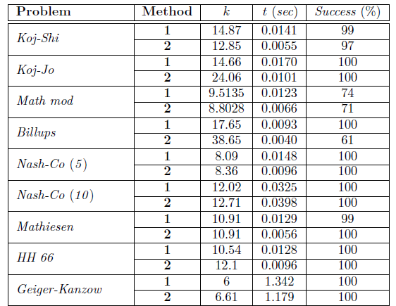
The results of Table 1 show that the number of iterations with Methods 1 and 2 are similar, except for two of the problems for which Method 2 increases them. In average time, except for one problem, Method 2 always is better (even with the problems where there are more iterations). In Succes(%), they are similar, except in the case of Billups Problem, where it decreases by 31 % with Method 2. Thus, for this set of numerical test, Method 1, generally used to choose λ in nonsmooth Newton-type methods for NCP, is not better than a random choice of this parameter (Method 2), which indicates that it would be convenient to find an alternative to choosing λ.
Now, we compare Algorithm 1 with Algorithms 2, 3, and 4. For this comparison, first, we consider Algorithm 1 with Method 1 versus the other three algorithms. Afterward, we consider Algorithm 1 with Method 2. We do numerical tests using the fixed starting points described previously. In addition, we take λ = 2 in our algorithm to obtain Algorithm 3 [18]. We measure the average of iterations and the average algorithm execution time. We present the results in Table 2.
To compare with Algorithm 2, we consider the results associate with Koj-Jo, Koj-Shi, Math mod, and Billups problems, which were also used in [5] to analyze the performance of its algorithm (Tabla 4.2 in [5]). Algorithm 1, with Methods 1 and 2, converges for some starting points for which Algorithm 2 does not converge. For example, with Method 1, the Koj-Jo problem with x 10 and the Billups problem with x14, and with Method 2, the Koj-Jo problem with x 20. To compare with Algorithm 3, we consider the results in Table 2 for Methods 1 and 2 versus those in the same table for λ = 2. We observe that with Method 1, the average number of iterations and the execution time of Algorithms 1 and 3 are similar. Now, Algorithm 3 compared to Algorithm 1 using Method 2 presents better performance for some problems in the average number of iterations, (Mathiesen and Geiger-Kanzow problems). On the other hand, the execution time with these two methods is very similar, except for 3 problems (Mathiesen Mod, Billups, H66), where it is less using Method 2. Thus, being able to choose A brings advantages.
Taking into account the results for Koj-Shi, Mathiesen, HH 66, and Geiger-Kanzow problems, reported in Table 2 for Algorithm 1 and in Tables 1 to 4 in [32] for Algorithm 4, we observe that in all cases, our algorithm with Methods 1 finds a solution in fewer iterations. However, with Method 2, it generally exceeds the number of iterations reported in [32].
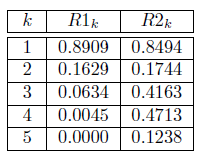
Finally, we analyze the local performance of Algorithm 1. In Section 6, we prove, under certain hypotheses, that Algorithm 1 converges superlinear and even quadratically, which is desirable for an iterative method. To illustrate this types of convergence we calculate the quotients
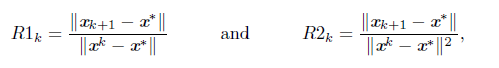
which are related to the definitions of superlinear and quadratic convergence of a vector sequence, respectively. In Table 3, we present the results for Billups problem (for more examples, see [30]). In this Table, R1 k , clearly, converges to zero, which means that Algorithm 1 converges at least superlinearly, and R2k seems to be bounded, which means that Algorithm 1 may converge quadratically. This fast convergence of Algorithm 1 is due to (closely related to what was proved in Section 6: near the solution, the Newton step is full (t k = 1). Moreover, this is illustrated in Table 4, where the column np indicates the full number of steps in the linear search which also correspond to the last steps.
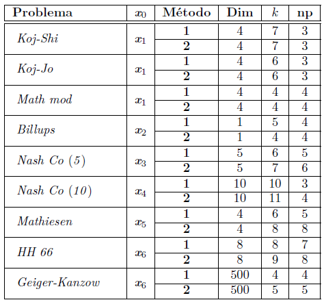
It is important to mention that in all cases, Algorithm 1 uses the Newton direction which is desirable because it makes its convergence fast. In the 77% of numerical tests, the number of full Newton steps in the monotone linear search (np) is greater than or equal to half the number of iterations ( k/2, ) which explains the fast convergence of our algorithm for this set of tests.
In the other part, we use three indices to collect additional information to compare Algorithm 1, varying λ (Methods 1 and 2) with Algorithm 3 (Algorithm 1 with λ = 2). These indices are the follows [6]:
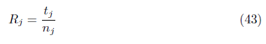
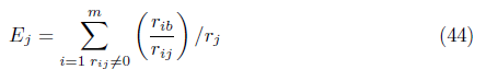
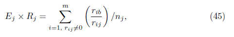
where r ij is the number of iterations required to solve the problem i by the method j, r ib = minj , t j is the number of successes by method j and nj is the number of problems attempted by method j.
For the calculation of the indices, we use the data from Table 4 and Table 7.1 in [30], the latter for λ - 2. In Table 5, we present the results obtained.
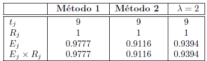
On this set of problems, the results in Table 5 confirm robustness of Algorithm 1 with the three choices of parameter λ. Also, the algorithm is more efficient with the dynamic choice of A (Method 1) of the three, although further testing will indicate to what extent this is true of broader classes of problems.
8. Final Remarks
One way to deal with the non-differentiability of the NCP is using the smoothed Jacobian strategy [9], [18], which allows us to approximate the reformulation of the problem by a succession of differentiable nonlinear systems that depend on a positive parameter. In this article, we proposed a global smoothed Jacobian algorithm that generalizes the one proposed in [18] to all members of the family defined in (5). We developed their convergence theory and did numerical tests to analyze their global and local performance. Our proposal presents some advantages in terms of global convergence compared to other methods as those proposed in [5], [18], and [32].
Finally, we believe that it is necessary to study a relationship between the parameter A and the nonlinear complementarity problem, which may improve the convergence of the algorithm. It would also be interesting to apply the smoothing Jacobian strategy to equation-reformulation of the nonlinear complementarity problem presented in [32].

