


 Inglés (pdf)
 Articulo en XML
 Referencias del artículo
 Enviar articulo por email
 Citado por SciELO
  Citado por Google
  Similares en
SciELO
Similares en
SciELO  Similares en Google
 Permalink
1. Introduction
The Kummer-Schwarz equation appears in various mathematical contexts like theory of functions, differential geometry, complex analysis, differential equations, integrable systems, mathematical physics, Sturm - Liouville equation, study of curves in a Lorentz space, the charge of density of dark energy [12, 32, 34]. In [26], Leach suggested several generalizations of the Kummer-Schwarz Equation (KS - 3):
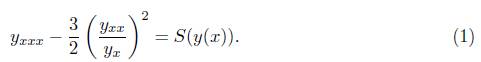
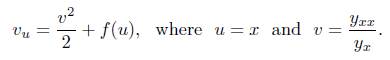
The generalizations before mentioned are important due to their connection to the Schwarzian derivative, (see Milne - Pinney [7]), the Riccati equations and its algebraic properties. The equation (1) has the Lie point symmetry algebra sl(2, ℝ) ⊕ sl(2, ℝ). The KS - 3 equation can be useful in the interpretation of physical systems; e.g., the case of quantum non-equilibrium dynamics of many body systems. The global dynamics of the Kummer - Schwarz differential equation was studied in [29]. Following this line, in [9, 18] considered a generalization of Kummer - Schwarz differential equation for KS - 3, namely
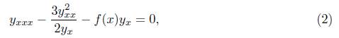
where f is an arbitrary function, they presented the group of symmetries

Such a symmetry group is a Non Solvable Lie Algebra and using this algebra, in [18] the following reduction is proposed for (2)
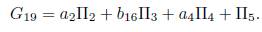
That is, it's corresponding Riccati equation. In [9, 20], was presented the group of Lie symmetries of (1), such symmetry group is (without explaining the details in their calculations)
Thus, in [20] the following solutions are proposed for (1)
these solutions are calculated using the method presented by Hydon [14], which proposes how to find a complete list of all discrete symmetry groups for a differential equation and its possible solutions. In [41], Polyanin and Zaitsev presented the following differential equation

Note that equation (2) is a particular case of equation (6) when f (x) = 0. For this equation they present the following solution

where C
1
,C
2
and C
3
are arbitrary constants. Using this solution proposed by [41] with A =
 , they got
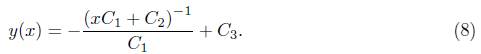
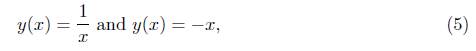
The objective of our work is: i) to provide a complete classification of Lie symmetries group for (2), ii) to present the optimal system (optimal algebra) for (1), iii) making use of all elements of the optimal algebra, to propose invariant solutions for (1) different from (5) and (8), finally iv) to classify the Lie algebra associated to (1), corresponding to the Lie symmetry group.
Lie group symmetry method is an interesting instrument employed to study different types of differential equations. This theory was introduced by the prominent Norwegian mathematician Sophus Lie [28] in the latter half of nineteenth century, following the idea of Galois theory in Algebra who clarified the relationship between the solution of polynomial equations and their symmetries. This method applied to differential equations continues to be useful in the fields of mathematics and applied physics and consequently new results are published an a regular basis. Its importance lies among many things to be built, for example, conservation laws using Noether's theorem [33]. In the same way, it is possible to construct invariant solutions for the differential equation understudy or a reduction of it, which with other traditional methods is not always possible. A huge reference in Lie group method can be found in the literature, e.g., [4, 8, 15, 36, 39].
Recently, the Lie group method approach has been applied to solve and analyze different problems in many scientific fields, e.g., in [25], the authors applied the Lie symmetry method to investigate some solutions for pZK equation, which models the nonlinear propagation of dust-ion acoustic solitary waves and shocks, and in [11] the authors studied the invariance of stochastic differential equations under random diffeomorphisms and established the determining equations for random Lie point symmetries of stochastic differential equations. Some references in the latest progress using Lie group symmetries can be found in [1, 10, 13, 27, 37, 40] and references therein, some recent publications in the area of Lie symmetry groups, optimal system, and invariant solutions can be found in [2, 21, 22, 23, 24, 30, 31, 38].
2. Lie Point Symmetries
In this section, we study the Lie point symmetries of (2). Following the classical Lie technique for calculating the symmetries of differential equations [6, 19, 35, 36], we carried out the complete group classification for (2). The corresponding result can be stated as follows.
Proposition 2.1. The Lie point symmetry group of the generalization of Kummer -Schwarz differentialequation (2)with arbitrary f, is generated by

for the special choices of f listed below (Table 1) we have,
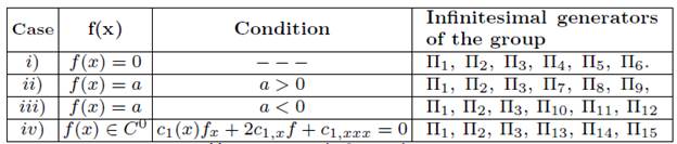
Where
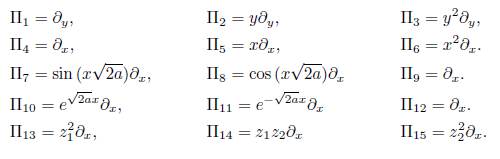
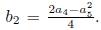
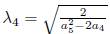
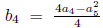
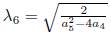
with z 1 ,Z 2 - linearly independent solutions of 2z" - f (x)z 0.
Proof. A general form of the one-parameter Lie group admitted by (2) is given by

where Є is the group parameter. The vector field associated with the group of transformations shown above can be written as
 . Applying its third prolongation
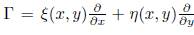
to (2), we must find the infinitesimals ξ(x, y), η(x,y) satisfying the symmetry condition
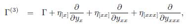
associated with (2). Here, η [x] , η [xx] and η [xxx] are the coefficients in Γ (3 given by
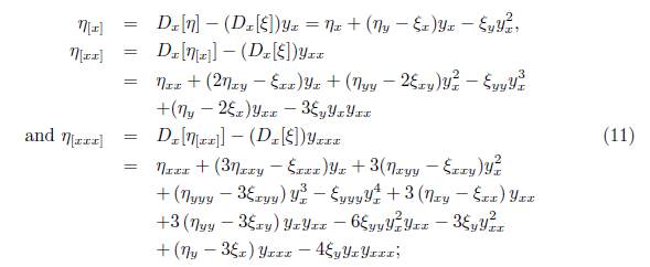
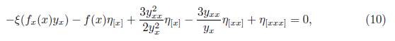
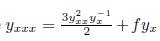
where D x is the total derivative operator: D x = ∂ x + y x ∂ y + y xx ∂ yx + y xxx ∂ yx Replacing (11) into (10) we obtain:
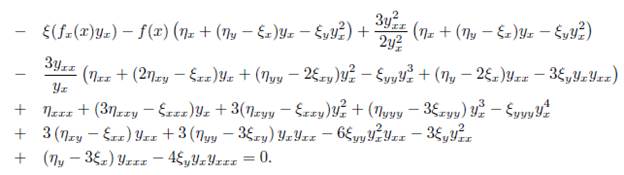
If we denote f ≅ f (x) and substitute
 in the last expression we have
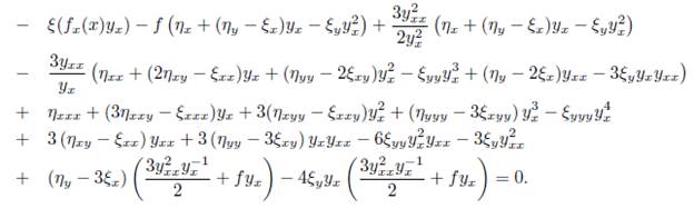
Thus, we can rearrange the last expression with respect to 1, y x , y 2 x , y 3 x , y 4 x ,y xx , y 2 xx , y −1 x y x x, y x y xx , y −1 x y 2 xx , y −2 x y xx and y −2 x y 2 xx and canceling some terms we obtainthe determining equations for the symmetry group of (2). That is:
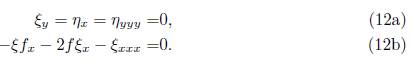
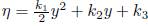
Solving in (12a), we have ξ = c1(x) and
 , with k
1
, k
2
, k
3
as arbitrary constants and c1(x) arbitrary function. If f is arbitrary then in (12b) we have ξ = 0 and
, with k
1
, k
2
, k
3
as arbitrary constants and c1(x) arbitrary function. If f is arbitrary then in (12b) we have ξ = 0 and
 , where and k
3
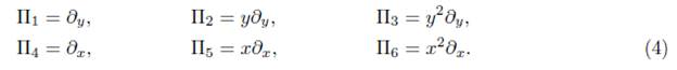
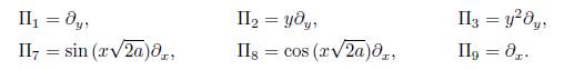
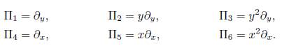
are arbitrary constants. Therefore the group of symmetries are Π1 = ∂
y
, Π2 = y
∂
y, Π3 = y
2
∂
y
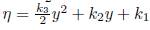
. This is consistent with What is presented in [18, 9]. If f = α # 0 where a is an arbitrary constant. Thus, we have two cases in (12b) which are α > 0 and α < 0.
, where and k
3
are arbitrary constants. Therefore the group of symmetries are Π1 = ∂
y
, Π2 = y
∂
y, Π3 = y
2
∂
y
. This is consistent with What is presented in [18, 9]. If f = α # 0 where a is an arbitrary constant. Thus, we have two cases in (12b) which are α > 0 and α < 0.
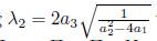
Case I: If α > 0 then in (12b) we have 2αξx + ξ
xxx
= 0 and solving for ξ we obtain
 where k7
, k8 and kg are arbitrary constants, then of (12a) we have
where k7
, k8 and kg are arbitrary constants, then of (12a) we have
 , Therefore the group of symmetries are
Case II: If α < 0 then in (12b) we have -2αξ
x
+ ξ
xxx
= 0 and solving for ξ we obtain
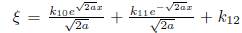 where k
10
,k
11
and k12 are arbitrary constants, then of (12a) we have
where k
10
,k
11
and k12 are arbitrary constants, then of (12a) we have
 . Therefore the group of symmetries are
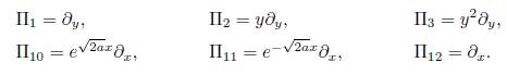
If f = 0 then in (12b) we have ξ
xxx
= 0 and solving for ξ we obtain
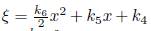 where k4, k5 and k
6
are arbitrary constants, then of (12a) we have
where k4, k5 and k
6
are arbitrary constants, then of (12a) we have
 . Therefore the group of symmetries are
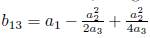
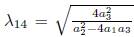
This is consistent with what is presented in [9, 20]. Let's remember that ξ = c1(x), then for the other cases of f in (126) the following differential equation must be satisfied c 1 (x)f x + 2c 1,x f + c 1¡xxx = 0, so, if the functions c1(x) and f (x) satisfy Eq. (126) then we have the following operator, additional to (9): X c1 = c1(x) ∂ x, therefore following [3] we have the solution is given in the terms of two linearly independent solutions of the associated to (126) homogeneous second-order Sturm-Liouville equation
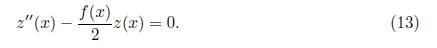
By the existence and uniqueness theorem if f (x) Є C 0 then there exists a nonzero solution z1 of Eq. (13). We look for another solution z2 of (13) such that
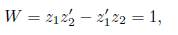
that is z 1 and z 2 are linearly independent solutions of (13) with Wronskian = 1 . Thus therefore following [3] we have the solution c1(x) = k13z1 2(x) + k14z1(x)z2(x) + k15z2(x), then it follows that for any f ЄC 0 there are three additional symmetries. Namely:

Thus, the demonstration of the Proposition 2.1 is finished. 0
3. Optimal Algebra
Taking into account [15, 17, 35, 42], we present in this section the optimal algebra associated to the symmetry group of (1), that shows a systematic way to classify the invariant solutions.
To obtain the optimal algebra, we should first calculate the corresponding commutator table, which can be obtained from the operator
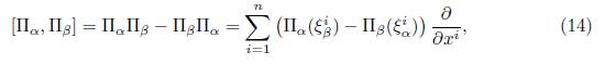
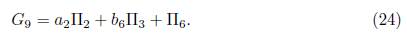
where i = 1, 2, with α, β = 1, • • • , 6 and ξ α i , ξ βi are the corresponding coefficients of the infinitesimal operators Π α ,Π β , . After applying the operator (14) to the symmetry group of (1), we obtain the operators that are shown in the following table
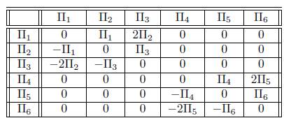
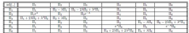
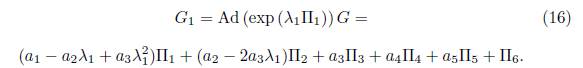
Now, the next thing is to calculate the adjoint action representation of the symmetries of (1) and to do that, we use Table 2 and the operator
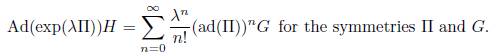
Making use of this operator, we can construct the Table 3, which shows the adjoint representation for each Πi.
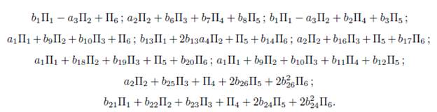
Proposition 3.1. The optimal algebra associated to the equation (1) is given by the vector fields
Proof. To calculate the optimal algebra system, we start with the generators of symmetries (1) and a generic nonzero vector. Let

The objective is to simplify as many coefficients α i as possible, through maps adjoint to G, using Table 3.
1) Assuming ae = 1 in (15) we have that G = α 1Π1+ α 2Π2+ α 3Π3+ α 4Π4+α 5Π5+Π6.Applying the adjoint operator to (Π1 ,G), we get
1.1) Case
 is eliminated, therefore G
1 = b
1Π1 +α
3Π3 + α
4Π4 + α
5Π5 +Π6 with
is eliminated, therefore G
1 = b
1Π1 +α
3Π3 + α
4Π4 + α
5Π5 +Π6 with
 . Now, applying the adjoint operator to (Π2
,G
1) we don’t have any reductions, thus applying the adjoint operator (Π3
,G
1) we get G
2 = Ad (exp (λ
2Π3))G
1 = b
1Π1+b
1
λ
2
2 Π2+( α
3+b
1
λ
2
2)Π3 + α
4Π4 + α
5Π5 + Π6.
. Now, applying the adjoint operator to (Π2
,G
1) we don’t have any reductions, thus applying the adjoint operator (Π3
,G
1) we get G
2 = Ad (exp (λ
2Π3))G
1 = b
1Π1+b
1
λ
2
2 Π2+( α
3+b
1
λ
2
2)Π3 + α
4Π4 + α
5Π5 + Π6.
1.1.A) Case
α
2
2
−4 α
1
# 0. Using
 with α
2
2
−4 α
1# 0, is eliminated Π3, thus G
2 = b
1Π1
− α
3Π2+ α
4Π4+ α
5Π5+Π6. Now, applying the adjoint operatorto (Π4
,G
2), we get
with α
2
2
−4 α
1# 0, is eliminated Π3, thus G
2 = b
1Π1
− α
3Π2+ α
4Π4+ α
5Π5+Π6. Now, applying the adjoint operatorto (Π4
,G
2), we get

Using
 is eliminated Π5, thus G3 = b1Π1
- α3Π2 + b2 Π4 + Π6, with
is eliminated Π5, thus G3 = b1Π1
- α3Π2 + b2 Π4 + Π6, with
 . Now applying the adjoint operator to (Π5, G
3 ), we don't have any reduction, but applying the adjoint operator to (Π6, G
3) we get
. Now applying the adjoint operator to (Π5, G
3 ), we don't have any reduction, but applying the adjoint operator to (Π6, G
3) we get

1.1.A.A1) Case
α
2
5
−2α
4
# 0. Using
 with α
2
5
−2α
4
# 0, is eliminated Π6. Then we have an element of the optimal algebra
with α
2
5
−2α
4
# 0, is eliminated Π6. Then we have an element of the optimal algebra

This is how a reduction of the generic element (15) ends.
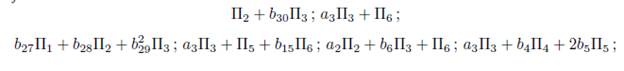
1.1.A.A 2 ) Case α 2 5 - 2α 4- = 0. Then we get b2 = 0, thus G4 = b1Π1 - α 3Π2 + Π6. Then we have an element of the optimal algebra

This is another way how a reduction of the generic element (15) ends.
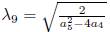
1.1.B) Case α 2 2 - 4α1 = 0. We get b1 = 0, thus G 2 = α 3Π3 + α 4Π4 + α 5Π5 + Π6. Now, applying the adjoint operator to (Π4 ,G 2), we have

Using
 , then Π 5 is eliminated, then we obtain G
5 = α
3Π3 + b
4Π4 + Π6, with
, then Π 5 is eliminated, then we obtain G
5 = α
3Π3 + b
4Π4 + Π6, with
 . Now applying the adjoint operator to (Π5
,G
5), we don’t have any reduction, but applying the adjoint operator to (Π6
,G
5) we have G
6 =Ad (exp (λ
6Π6))G
5 = α
3Π3 + b
4Π4 + 2b
4
λ
6Π5 + (2λ
2
6
b
4 + 1)Π6
.
. Now applying the adjoint operator to (Π5
,G
5), we don’t have any reduction, but applying the adjoint operator to (Π6
,G
5) we have G
6 =Ad (exp (λ
6Π6))G
5 = α
3Π3 + b
4Π4 + 2b
4
λ
6Π5 + (2λ
2
6
b
4 + 1)Π6
.
1.1.B.B1) Case
α
2
5
−4α
4
# 0. Using
 with α
2
5
−4α
4
# 0, is eliminated Π6. Then we have an element of the optimal algebra
with α
2
5
−4α
4
# 0, is eliminated Π6. Then we have an element of the optimal algebra

This is how a reduction of the generic element (15) ends.
1.1.B.B2) Case α 2 5 − 4α 4 = 0. We get b 4 = 0, then we have an element of the optimal algebra

This is how a reduction of the generic element (15) ends.
1.2) Case
α
3 = 0. We get, G
1 = (α
1
− α 2λ1)Π1 + α
2Π2 + α
4Π4 + α
5Π5 + Π6. 1.2.A) Case
α
2
# 0. Using
 , with α
2 # 0, is eliminated Π1, thus we get G
1 = α
2Π2 + α
4Π4 + α
5Π5 + Π6. Now, applying the adjoint operator to (Π2
,G
5) and (Π5
,G
5), we don’t have any reduction, then applying the adjoint operator to (Π3
,G
1) we get G
7 = Ad (exp (λ
7Π3))G
1 = α
2Π2 + α
2
λ
7Π3 + α
4Π4 + α
5Π5 +Π6, it is clear that we don’t have any reduction, then we have G
7 = α
2Π2+b
6Π3+ α
4Π4+ α
5Π5 +Π6, with b
6 = α
2
λ
7. Now, applying the adjoint operator to (Π4
,G
7) we get G
8 = Ad (exp (λ
8Π4))G
7 = α
2Π2+b
6Π3+( α 4− α
5
λ
8+λ
2
8 )Π4+( α
5
−2λ
8)Π5+Π6. Using
, with α
2 # 0, is eliminated Π1, thus we get G
1 = α
2Π2 + α
4Π4 + α
5Π5 + Π6. Now, applying the adjoint operator to (Π2
,G
5) and (Π5
,G
5), we don’t have any reduction, then applying the adjoint operator to (Π3
,G
1) we get G
7 = Ad (exp (λ
7Π3))G
1 = α
2Π2 + α
2
λ
7Π3 + α
4Π4 + α
5Π5 +Π6, it is clear that we don’t have any reduction, then we have G
7 = α
2Π2+b
6Π3+ α
4Π4+ α
5Π5 +Π6, with b
6 = α
2
λ
7. Now, applying the adjoint operator to (Π4
,G
7) we get G
8 = Ad (exp (λ
8Π4))G
7 = α
2Π2+b
6Π3+( α 4− α
5
λ
8+λ
2
8 )Π4+( α
5
−2λ
8)Π5+Π6. Using
 , is eliminated Π5, the we have G
8 = α
2Π2 + b
6Π3 + b
7Π4 + Π6, with
, is eliminated Π5, the we have G
8 = α
2Π2 + b
6Π3 + b
7Π4 + Π6, with
 . Now, applying the adjoint operator to (Π6
,G
8) we get G
9 =Ad (exp (λ
9Π6))G
8 = α
2Π2 + b
6Π3 + b
7Π4 + 2b
7
λ
9Π5 + (2b
7
λ
2
9 + 1)Π6.
. Now, applying the adjoint operator to (Π6
,G
8) we get G
9 =Ad (exp (λ
9Π6))G
8 = α
2Π2 + b
6Π3 + b
7Π4 + 2b
7
λ
9Π5 + (2b
7
λ
2
9 + 1)Π6.
1.2.A.A1) Case
α
2
5
−4α
4
# 0. Using
 with α
2
5
−4α
4
# 0, is eliminated Π6. Then we have an element of the optimal algebra
with α
2
5
−4α
4
# 0, is eliminated Π6. Then we have an element of the optimal algebra

This is how a reduction of the generic element (15) ends.
1.2.A.A2) Case α2 5 - 4α 4- = 0. We get b7 = 0, then we have an element of the optimal algebra
This is how a reduction of the generic element (15) ends.
1.2.B) Case α 2 = 0. We get G 1 = α 1Π1 + α 4Π4 + α 5Π5 + Π6. Now, applying the adjoint operator to (Π2 ,G 5) and (Π5 ,G 5), we don’t have any reduction, then applying the adjoint operator to (Π3 ,G 1) we get G 10 = Ad (exp (λ 10Π3))G 1 =α 1Π1 +2α 1 λ 10Π2 +α 1 λ 10Π3 +α 4Π4 +α 5Π5 +Π6, it is clear that we don’t have any reduction, then we have G 10 = α 1Π1 + b 9Π2 + b 10Π3 + α 4Π4 + α 5Π5 + Π6, with b 9 = 2α 1 λ 10 and b 10 = α 1 λ 10.
Now, applying the adjoint operator to (Π4
,G
10) we get G
11 =Ad (exp (λ
11Π4))G
11 = α
1Π1 + b
9Π2 + b
10Π3 + (α
4
− α
5
λ
11 + λ
2
11)Π4 + (α
5
− 2λ
11)Π5 + Π6. Using
 , is eliminated Π5, then we have G
11 = α
1Π1 + b
9Π2 + b
10Π3 + b
11Π4 + Π6, with
, is eliminated Π5, then we have G
11 = α
1Π1 + b
9Π2 + b
10Π3 + b
11Π4 + Π6, with
 .
.
Now, applying the adjoint operator to (Π6 ,G 11) we get G 12 =Ad (exp (λ 12Π6))G 11 = α 1Π1+b 9Π2+b 10Π3+b 11Π4+2b 11 λ 12Π5+(2b 11 λ 2 12+1)Π6.
1.2.B.A
1) Case 4α
4
− α
2
5
# 0. Using
 , is eliminated Π6, then wehave an element of the optimal algebra

This is how a reduction of the generic element (15) ends.
1.2.B.A 2) Case 4α 4 −α 2 5 = 0. We get b 11 = 0, thus we have G 12 = α 1Π1 +b 9Π2 +b 10Π3 + Π6, then we have an element of the optimal algebra

This is how a reduction of the generic element (15) ends.
2) Assuming α 6 = 0 and α 5 = 1 in (15) we have that G = α 1Π1 + α 2Π2 + α 3Π3 + α 4Π4 + Π5. Applying the adjoint operator to (Π2 ,G) and (Π5 ,G) we don’t haveany reduction, thus applying the adjoint operator to (Π1 ,G) we get
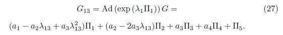
2.1) Case α3 # 0. Using
 with α3 # 0, is eliminated Π 2, we get
 . Then using
 , we have G
13 = b
13Π1 + α 3Π3 + α 4Π4 + Π5. Now, applying the adjoint operator (Π3, G
13), we have
, we have G
13 = b
13Π1 + α 3Π3 + α 4Π4 + Π5. Now, applying the adjoint operator (Π3, G
13), we have

2.1.A) Case 4 α 1 α 3
- α2
2 =0. Using
 is eliminated Π3, the we get G14 = b13 Π1 + 2b13λ14 Π 2 + α
4
Π
4
+ Π 5. Now applying the adjoint operator to (Π 4,G14), we have:
is eliminated Π3, the we get G14 = b13 Π1 + 2b13λ14 Π 2 + α
4
Π
4
+ Π 5. Now applying the adjoint operator to (Π 4,G14), we have:

Using λ 15 = α 4, is eliminated Π4, then G 15 = b 13Π1+2b 13 α 4Π2+Π5 . Now applying the adjoint operator to (Π6 ,G 15), we have:

We don't have any reduction, then we have an element of the optimal algebra

With b 14= λ 16. This is how a reduction of the generic element (15) ends.
2.1. B) Case 4α1α3 - α2 2 , =0. We get b13 = 0, then G 14 = α 3Π3 + α 4Π4 + Π5. Now applying the operator to (Π4 ,G 14) we have

Using λ 17 = α 4, is eliminated Π4, then we have G 17 = α 3Π3 + Π5 . Now using the operator to (Π6 ,G 17), we get:

We don't have any reduction, then using λ18 = b15, we have an element of the optimal algebra

This is how a reduction of the generic element (15) ends.
2.2) Case α3 = 0. We get G 13 = (α 1 − α 2 λ 13)Π1 + α 2Π2 + α 4Π4 + Π5.
2.2.A1) Case α2
# 0. Using
 , with α
2 0, is eliminated Π1, then we have G
13 = α
2Π2 + α
4Π4 + Π5. Now applying the operator to (Π3
,G
13) we have G
19 = Ad (exp (λ
19Π3))G
13 = α
2Π2 + α
2
λ
19Π3 + α
4Π4 + Π5
. It is clear that we don’t have any reduction, then using b
16 = α
2
λ
19 we get
, with α
2 0, is eliminated Π1, then we have G
13 = α
2Π2 + α
4Π4 + Π5. Now applying the operator to (Π3
,G
13) we have G
19 = Ad (exp (λ
19Π3))G
13 = α
2Π2 + α
2
λ
19Π3 + α
4Π4 + Π5
. It is clear that we don’t have any reduction, then using b
16 = α
2
λ
19 we get
Now applying the operator to (Π4 ,G 19) we get: G 20 = Ad (exp (λ 20Π4))G 20 =α 2Π2 + b 16Π3 + (α 4 − λ 20)Π4 + Π5 . Then using λ 20 = a 4, is eliminated Π4, thus G 19 = α 2Π2 + b 16Π3 + Π5 . Now applying the operator (Π6 ,G 20), we get

It is clear that we don't have any reduction. The using λ 21 = b 17 , we have an element of the optimal algebra

This is how a reduction of the generic element (15) ends.
2.2.A2) Case α2 = 0. We get G13 = α 1Π1+ α 4Π4+Π5. Now applying the operator to (Π3, G 13) we have

we don't have any reduction, then using b18 = 2α1λ22 and b19 = α1λ2 22, we obtain
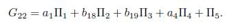
Now, applying the operator to (Π4, G 22) we have

Using λ23 = α4, is eliminated II4 then we get G23 = α 1 Π 1 + b18 Π2 + b1g Π3 + Π5. Now applying the operator to (Π3, G23) we have

It is clear that we don't have any reduction, then using λ24 = b20, we have an element of the optimal algebra

This is how a reduction of the generic element (15) ends.
3) Assuming α 3 = α 5 =0 and α 4 = 1 in (15), we have that G = α 1 Π 1 + α 2 Π2 + α 3Π3 + Π4. Applying the adjoint operator to (Π2,G), (Π 4 ,G) and (Π5,G) we don't have any reduction, on the other hand applying the adjoint operator to (Π1 , G) we get

3.1) Case
α
3
# 0. Using
 with α3 # 0, in (32), Π2 is liminated, therefore G
25 = b
21Π1 + α
3Π3 + Π4, with b
21 = α
1 + 2λ
25 + α
3
λ
2
25. Now, applying the adjoint operator to (Π3
,G
25), we get G
26 = Ad (exp (λ
26Π3))G
25 = b
21Π1 +2b
21
λ
26Π2 + (α
3 + b
21
λ
2
26)Π3 + Π4. It is clear that we don’t have any reduction, then G
26 = b
21Π1 +b
22Π2 +b
23Π3 +Π4, with b
22 = 2b
21
λ
26 and b
23 = α
3 +b
21
λ
2
26. Now applying the adjoint operator to (Π6
,G
26) we have
with α3 # 0, in (32), Π2 is liminated, therefore G
25 = b
21Π1 + α
3Π3 + Π4, with b
21 = α
1 + 2λ
25 + α
3
λ
2
25. Now, applying the adjoint operator to (Π3
,G
25), we get G
26 = Ad (exp (λ
26Π3))G
25 = b
21Π1 +2b
21
λ
26Π2 + (α
3 + b
21
λ
2
26)Π3 + Π4. It is clear that we don’t have any reduction, then G
26 = b
21Π1 +b
22Π2 +b
23Π3 +Π4, with b
22 = 2b
21
λ
26 and b
23 = α
3 +b
21
λ
2
26. Now applying the adjoint operator to (Π6
,G
26) we have

It is clear that we don't have any reduction, then using λ27 = b24, we have other element of the optimal algebra

This is how other reduction of the generic element (15) ends.
3.2) Case
α
3 = 0. We get G
25 = (α
1
− 2λ
25)Π1 + α
2Π2 + Π4, using
 , is eliminated Π1, thus G
25 = α
2Π2 + Π4. Now applying the adjoint operator to (Π3
,G
25) we get:
, is eliminated Π1, thus G
25 = α
2Π2 + Π4. Now applying the adjoint operator to (Π3
,G
25) we get:

we don’t have any reduction, then using α 2 λ 28 = b 25, we obtain G 28 = α 2Π2 +b 25Π3 + Π4 . Now applying the adjoint operator to (Π6 ,G 28) we have:

It is clear that we don't have any reduction, then using λ 29 = b 26, we have other element of the optimal algebra

4) Assuming α6 = α5 = α4 = 0 and α3= 1 in (15), we have that G = α 1Π1+α 2Π2+Π3. Applying the adjoint operator to (Π2 ,G), (Π4 ,G), (Π5 ,G) and (Π6 ,G) we don’t have any reduction, on the other hand, applying the adjoint operator to (Π1 ,G) we get

Using
 , in (35), is eliminated Π2, therefore G30 = b27 Π1 + Π3, with
 . Now, applying the adjoint operator to (Π3,G30) we get:

Then, we don't have any reduction, thus using b28 = 2b27λ31 and b29 = 1 + λ2 31, we have other element of the optimal algebra

This is how other reduction of the generic element (15) ends.
5) Assuming α6 = α5 = α4 = α3 = 0 and α2 = 1 in (15), we have that G = α1 Π1 + Π2. Applying the adjoint operator to (Π2, G), (Π4, G), (Π5, G) and (Le, G) we don't have any reduction, on the other hand, applying the adjoint operator to (Π1 , G) we get

Using λ 32 = α1 , is eliminated Π1 , thus we get G 32 = Π2. Now applying the adjoint operator to (Π3, G 32), we have

We don't have any reduction, then using λ 33 = b 30 we have other element of the optimal algebra

This is how other reduction of the generic element (15) ends.
6) Assuming α 6 = α 5 = α 4 = α 3 = α 2 = 0 and α 1 = 1 in (15), we have that G = Π1. Applying the adjoint operator to (Π1 , G), (Π2, G), (Π3, G), (Π4, G), (Π5, G) and (Π6 , G) we don't have any reduction, on the other hand, applying the adjoint operator to (Π3, G) we get

It is clear that we don't have any reduction, then using λ 34 = b 31 we have other element of the optimal algebra

This is how other reduction of the generic element (15) ends.
4. Invariant solutions by generators of the optimal algebra
In this section, we characterize all invariant solutions taking into account some operators that generate the optimal algebra presented in Proposition 3.1. For this purpose, we use the method of invariant curve condition [15] (presented in section 4.3), which is given by the following equation

Using the element Π2+Π3 from Proposition 3.1, under the condition (41), we obtain that Q = η
1
− yxξ
1 = 0, which implies (y + y
2) − y
x
(0) = 0, then solving this ODE we have
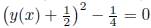 , which is trivial solution for (2) with y(x) = 0 or y(x) = −1, using an analogous procedure with all of the elements of the optimal algebra (Proposition 3.1), we obtain both implicit and explicit invariant solutions that are shown in the Table 4, with c being a constant.
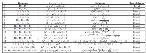
Remark 1. The column three in Table 4 which contain the solutions for Q(x, y,y x ), was calculated using by symbolic software: Mathematica.
5. Classification of Lie algebra
In the theory of finite dimensional Lie algebra it is possible to classify the Lie algebra by using the Levi's theorem, which state that any finite dimensional Lie algebra can be write as a semidirect product of a semisimple Lie algebra and a Solvable Lie algebra, that means that, the classification of Lie algebras reduces to the classification of the Solvable and semisimple Lie algebra. In the case of a semisimple Lie algebra (see [16]) we can use the Cartan's criterion to state if a Lie algebra is or not semisimple.
Let g the Lie algebra related to the symmetry group of infinitesimal generators of the equation (1) as stated by the table of the commutators, it is enough to consider the no vanish brackets: [Π1 ,Π2] = Π1, [Π1 ,Π3] = 2Π2, [Π2 ,Π3] = 2Π3, [Π4 ,Π5] = Π4, [Π4 ,Π6] = 2Π5, [Π5 ,Π6] = Π6, Using that we calculate Cartan-Killing form K as follows.
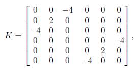
which the determinant is not zero, and thus by Cartan’s criterion this Lie algebra is semisimple. First, We remark that in the special lineal algebra sl(2, ℝ) with basis X, Y and H, we have the relations [X, Y ] = H, [X,H] = 2X [Y,H] = −2Y . Next, notice that if we use the transformation: X 1: = Π1 , Y 1: = Π3 H 1 = 2Π2, X 2: = Π4 , Y 2: = Π6 H 2 = 2Π5. From that we can see that X 1 , Y 1 ,H 1 and X 2 , Y 2 ,H 2 generate a three dimensional Lie algebra which are isomorphic each one to the special linear Lie algebra sl(2, ℝ). In fact since [X 1 ,H 1] = 2x 1, [X1, Y 1] = H1, [Y 1 ,H 1] = −2Y 1, and [X 2 ,H 2] = 2x 2, [X 2 , Y 2] = H 2, [Y 2 ,H 2] = −2Y 2, that is we have the same structure constants that the Lie algebra sl(2, ℝ), and since the structure constant classify the Lie algebra up isomorphism we obtain the complete classification of the Lie algebra g. In general terms we can write a element of the Lie algebra as Z = X+Y where X ∈ sl(2, ℝ) and Y ∈ sl(2, ℝ). Consequently, we have the next proposition
Proposition 5.1. The 6-dimensional Lie algebra g related to the symmetry group of the equation (1) is isomorphich with sl(2, ℝ) ⊕ sl(2, ℝ) .
6. Conclusion and future works
We obtained the complete classification of the group of symmetries of (2) (see Proposition 2.1) and using the Lie symmetry group (see Proposition 2.1 item i)), we calculated the optimal system, as it was presented in Proposition 3.1. Using these operators it was possible to characterize all the invariant solutions (see Table 4), these solutions are different from (5) and (8), so these solutions do not appear in the literature known until today. The Lie algebra associated to the equation (1) is isomorphic to sl(2, R) ©sl(2, R). Therefore, the goal initially proposed was achieved.
For future works, by classifying the group of symmetries it is possible to think about: to calculate the conservation laws using the Ibragimov method, to calculate the equivalence group associated with the complete classification, to get the Contact symmetries, Dynamic symmetries, Hidden symmetries and Lambda-symmetries associated with each group in the respective classification. On the other hand, the solutions obtained in Table 4, can be used to test the solution and convergence of numerical methods for this equation.

