1. Introduction

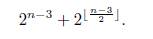
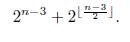
The Caterpillar trees were initially studied by F. Harary and A. J. Schwenk [¹] in a series of articles. The name was introduced by Arthur Hobbs, an American mathematician. In 1973, F. Harary and A.J. Schwenk [¹] showed that the number of nonisomorphic caterpillars with n ≥ 2 edges is 2 ⁿ⁻³ + 2 ^{⌊(n−3)/2⌋.} They found this formula in two ways: first, derived as a special case of an application of Pólya’s enumeration Theorem which counts graphs with integer-weighted points; secondly, by an appropriate labelling of the lines of the caterpillar. In this paper, we gave a new proof of this result using a new sum of graphs, introduced in [³, ²] and studied with great attention in [⁴].

The paper is organized as follows. In Section 2, we study a combinatorial problem which will be used in the proof of the main Theorem (see Theorem 3.7). In Section 3, we introduce the sum of graphs and use it to build the caterpillar trees, and, thus, give a new proof of the formula enumerating caterpillar trees on n ≥ 2 edges.

2. Combinatorial lemma

Let 𝔹 = {0, 1} and B ^m = 𝔹× · · · × 𝔹 the m-times Cartesian product of 𝔹. We define the following functions:

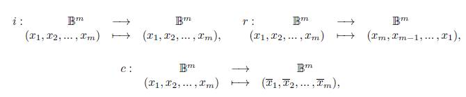
where, for k = 1, . . . , m,

Here, we consider for all f, g: 𝔹 ^m −→ 𝔹 ^m the composition f ◦ g: 𝔹 ^m −→ 𝔹 ^m .

Proposition 2.1. Let i, r, c: 𝔹 ^m −→ 𝔹 ^m be the functions defined above and take x ∈ 𝔹 ^m . Then, the following properties hold:

Proof. By definition of i, r and c, it is clear that (1), (2), (3) and (4) follows. And (5) follows from (4), (2) and (3).

Definition 2.2. Let x, y ∈ 𝔹 ^m . We will say that x is related to y when i( x ) = y or r( x ) = y or c( x ) = y or (c ◦ r)( x ) = y , and it will be denoted by x ∼ y .

Remark 2.3. The relation defined in Definition 2.2 is an equivalence relation.

In this section we prove the following combinatorial lemma for the equivalence classes associated with points in 𝔹 ^m .

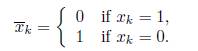
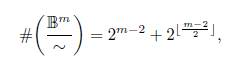
Lemma 2.4 (Combinatorial Lemma). Let x ∈ 𝔹 ^m and set [ x ] = {y ∈ 𝔹 ^m | x ∼ y}. Then,

Where and ⌊z⌋ is the largest integer smaller than or equal to z.

Proof.First, let’s show the following: The class [ x ] has 2 or 4 representatives.

Indeed, if x , r( x ), c( x ) and (c ◦ r)( x ) = (r ◦ c)( x ) are different from each other, we will get that the class [ x ] has 4 representatives, namely

On the other hand:

The cases i) and ii) have only 2 representatives for the class [ x ] and the affirmation follows.

Remark: x # c( x ) by definition.

Now, let be a class that only has 2 representatives. Set x = (x1, x2, · · · , xm). We have the following cases:

I) If x = r( x ) then

II) If x = (r ◦ c)( x ) then

In case (I), if m is even, we have to know the first entries of x = (x ₁ , x ₂ , · · · , x _m ), that is, we can form elements. Now, as pairwise elements belong to the same class, we have that belong to the same class, and, therefore, we will have two representatives. On the other hand, if m is odd, we first delete the central coordinate of x , to obtain the m − 1 even case, which leads us to have classes with two representatives. Now, considering the central coordinate of x , we see that it can take the values 0 or 1, and thus, when m is odd there are classes with two representatives.

Analogously, we have a similar result in case (II) when m is even. Note that when m is odd there are no representatives, since no x with m odd entries satisfies this case.

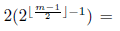
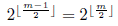
So, from (I) and (II), if m is even, we get 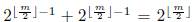classes with two representatives each. If m is odd, we get . Therefore, in both cases we have the same number of representatives.

The next step consists of computing . It follows from the Affirmation that ismade up of classes that have 2 or 4 elements. Thus, we can divide 𝔹m into a collectionof disjoint classes of 2 or 4 elements each. Thus, one gets

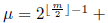
where μ is the number of classes of with two representatives, namely and η is the number of classes of with four representatives. Then, substituting these values in (1), one gets

Therefore,

3. Sum of graph and Caterpillar tree

Let us denote by A the set of all tree graphs.

The sum of graphs in A is an operation that is performed between two graphs of 𝔸. This sum is defined as follows:

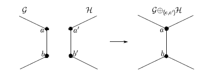
Definition 3.1. Let G = (V, E) and ℋ = (V ^′ , E ^′ ) be distinct graphs in A and let e = (a, b) ∈ E and e ^′ = (a ^′ , b ^′ ) ∈ E ^′ be edges. Then,

is a new graph such that e and e ^′ and their respective vertices, connecting G and ℋ, are identified. The graph G ⊕ _{e,e ′ _} ℋ is the sum between G and ℋ. This sum will be denoted by G ⊕ H if there is no confusion in the identification of the edges. See Figure 1 for a graphical representation of this sum.

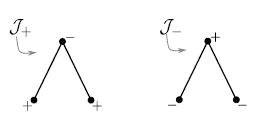
Definition 3.2. Consider the path P ₃ and J = P ₃. We denote by J ₊ the graph derived of J with two positive signs in the extreme vertices and a negative sign in the middle vertex, and by J ₋ to the graph derived of J with two negative signs in the extreme vertices and a positive sign in the middle vertex. See Figure 2.

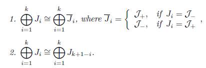
Definition 3.3. Let {J _i } ^k _i=1 be a family of graphs, where J _i ∈ {J ₊ , J ₋ }. We define J ₁ ⊕ J ₂ ⊕… ⊕ Jk, as follows:

We note that the identification of edges should be done while preserving the signs.

Notation. Given {J_i}^k _{i =1}, where J _i ∈ {J ₊ ,J ₋ }, we will denote by ⊕ ^k _i=1 J _i the sum J ₁⊕ .. ⊕ J _k in Definition 3.3. Thus: ⊕ ^k _i=1 J _i = J ₁⊕ … ⊕Jk. By convention,⊕⁰ _i=1 J _i = I, where I, is the graph of one edge.

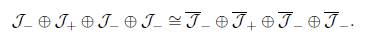
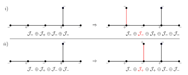
Example 3.4. InFigure 3 (i), we have the construction of J+ ⊕ J+ and J− ⊕ J−, according to the Definition 3.3, where we can see that J+ ⊕ J+ ≈ J− ⊕ J−, as graphs. Similarly, inFigure 3 (ii) we have the construction of J+ ⊕J− and J− ⊕J+, where we can see that J+ ⊕ J−⊕=J− ⊕ J+.

Proposition 3.5. Let {J _i } ^k _{i =1} be a family of graphs such that Ji 2 {J ₊ ,J ₋ }. Then, the following statements holds:

Proof. For (1), since J+≅J ₋ we have J _i ≅J _i for all i = 1, … , k. Then, if we replace J _i by J _i in ⊕ ^k _i=1 J _i we get ⊕ ^k _i=1 Ji and since the sums of the graphs continue to beperformed on the same edges, we have ⊕ ^k _i=1 J _i ≅⊕ ^k _i=1 Ji, see Figure 4.

For (2), we note that the sum ⊕ ^k _i=1 J _i = J ₁⊕J ₂⊕ … ⊕J _k−1 ⊕J _k is built starting from J ₁ which is added to J ₂ to obtain J ₁ ⊕ J ₂, latter we added J ₃ to obtain J ₁ ⊕ J ₂ ⊕ J ₃, and, thus, until we get the sum of J ₁ ⊕ J ₂ ⊕ … ⊕ J _k−1 and Jk to finally get J ₁ ⊕J ₂⊕ …⊕J ^k−1 ⊕ Jk = ⊕ ^k _i=1 J _i , but we also noted that this same sum is built as the sum of J _k and J _k−1 , and, thus, until we get to add J _k ⊕ … ⊕J ₂ with J ₁ to get J _k ⊕J _k−1 ⊕ … ⊕J ₂ ⊕J ₁ = ⊕ ^k _i=1 J _k+1−i . Thus, ⊕ ^k _i=1 J _i ≅ ⊕ ^k _i=1 J _k+1−i .

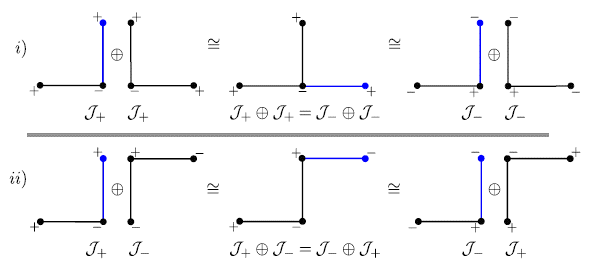
Example 3.6. The graphs J ₊ ⊕J ₋ ⊕J ₊ ⊕J ₊ and J ₋ ⊕J ₊ ⊕J ₋ ⊕J ₋ are built in (i) and (ii) ofFigure 4, respectively. Furthermore, 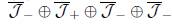and, thus:

The following Theorem is the main result of the paper (it was initially showed by F.

Harary and A.J. Schwenk in [1]), for which we gave an alternative proof.

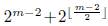
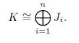
Theorem 3.7. Let 𝕁 = {J ₁ ⊕ · · · ⊕ J _i ⊕ · · · ⊕ J _m ∈ 𝔸 | J _i = J ₊ or J _i = J ₋ , ∀i = 1, · · · , m, and m ∈ ℕ }. Then, the number of different nonisomorphic graphs with n ≥ 2 edges in 𝕁, is given by

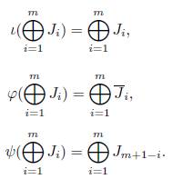
Proof. Given m ∈ ℕ, we define the functions ι, φ, ψ: 𝕁 → 𝕁 by

We say that ⊕ ^m _i=1 Ji and ⊕ ^m _i=1 L _i are ∼ _m related in 𝕁, denoted by

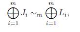
if

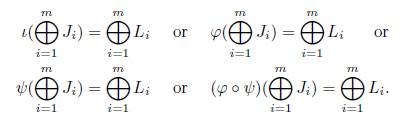
Now, we affirm that the relation ∼ _m is an equivalence relation. Indeed, it follows immediately by the combinatorial Lemma (Lemma 2.4), where we take J _i = x _i , J+ = 1, J− = 0, ⊕ ^m _i=1 J _i = (x ₁ , …, x _m ) and ι = i, φ = f, ψ = g, ∼m=∼. Furthermore,

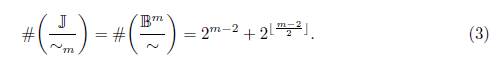
Thus, we have different graphs of the form ⊕ ^m _i=1 J _i , where J _i ∈ {J ₊ ,J ₋ }. Since the graphs ⊕ ^m _i=1 J _i have m + 1 edges, making n = m + 1 and substituting in (3) we have that the number of nonisomorphic different graphs, with n ≥ 2 edges in 𝕁, is given by

Given a Caterpillar tree fixed, the following result allows us to obtain a family {J _i } ^k _{i =1} , where J _i ∈ {J ₊ ,J ₋ }, such that K≅⊕ ^k _i=1 J _i .

Proposition 3.8. Let n be a positive integer and K be a Caterpillar tree with n + 1 edges, then there exists a family {J _i } ⁿ _i=1 , where J _i ∈ {J ₊ , J ₋ }, such that

Proof. By induction on the number E of edges of K.

For a graph with 1 edge, then by convention we have K≅⊕⁰ _i=1 J _i .

For a graph with 2 edges, we take K≅⊕¹ _i=1 J _i , where J _i = J ₊ or J _i = J ₋ .

Suppose that it is true for a graph with n edges, then K≅⊕ ⁿ⁻¹ _i=1 J _i .

Now, we show that it is true for a graph with n + 1 edges. Indeed, K′ is the graph that is obtained when deleting an end edge from K. Thus, K′ has E′ = edges. Then, by induction, we have that K′ ≅⊕ ⁿ⁻¹ _i=1 J _i . Now, in ⊕ ⁿ⁻¹ _i=1 J _i we insert an end edge by adding conveniently J+ or J−, so that ⊕ ⁿ _i=1 J _i ≅K as follows: first, we identify the sign of the vertex where the edge will be inserted (it is clear that said vertex is positive or negative). Then there will be a j such that ⊕ ⁿ⁻¹ _i=1 J _i = (⊕ ^n−1−j _i=1 J _i ) _ (⊕ ⁿ⁻¹ _i=n−j J _i ) so that the last vertex to the right of⊕ ^n−1−j _i=1 J _i become the vertex where the missing edge will be inserted. If the vertexis positive (resp. negative) we immediately add⊕ ^n−1−j _i=1 J _i with J− (resp. J ₊), andadding ⊕ ⁿ⁻¹ _i=n−j J _i , we get (⊕ ^n−1−j _i=1 J _i ) ⊕ J ₋ ⊕ (⊕ ⁿ⁻¹ _i=n−j J _i ) (resp. (⊕ ⁿ⁻¹⁻ _ji=1 J _i ) ⊕ J ₊ ⊕ (⊕ ⁿ⁻¹ _i=n−j ^J _i )). As was inserted the missing edge to ⊕ ⁿ⁻¹ _i=1 J _i to be isomorphic to K, we have that

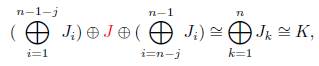
where J = J ₋ , if the last vertex created in ⊕ ^n−1−j _i=1 J _i has a positive sign and J = J+, if the last vertex created in ⊕ ^n−1−j _i=1 J _i has a negative sign.

An example for Proposition 3.8 is given in Figure 5.

Theorem 3.9. Let 𝕁₀ be the set of all different nonisomorphic graphs in 𝕁 and let 𝕂 be the set of nonisomorphic Caterpillar trees, then

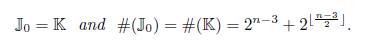
Proof. By Definition 3.3 we have that the graphs in 𝕁₀ are Caterpillar trees (thus 𝕁₀ ⊆ 𝕂) then, by Proposition 3.8, we get that every Caterpillar tree is isomorphic to an element of J₀, thus 𝕂 ⊆ 𝕁₀ and therefore 𝕁₀ = 𝕂. Furthermore,