


 Inglês (pdf)
 Artigo em XML
 Referências do artigo
 Enviar este artigo por email
 Citado por SciELO
  Citado por Google
  Similares em
SciELO
Similares em
SciELO  Similares em Google
 Permalink
1. Introduction
In recent years we have seen many applications of fractal sets in modeling sciences. Especially, to study several processes that can be modeled using fractals and specially self-similar structures. We mention processes related to diffusion on fractal sets witch have several possible applications, including diffusion of substances in biological structures and flow inside fractures in modeling fluid flow in fractured porous media, among other models. See [6, 9]. In this paper, we consider fractals defined as self-similar sets with the additional properties of being post-critically finite; see [6]. These self-similar sets can be approximated (in the Hausdorff metric) by a finite union of sets generated by removing a finite number of vertices from a graph approximation of the fractal set.
We recall the definition of the Laplace operator, a standard model for fractal diffusion. Then, introduce numerical approximation procedures of the presented model. It is im-portant to stress that our approximation procedure consists of renormalizing standard approximation methods on two- and three-dimensions such as the finite difference and the finite element method. See for example [3] where a finite element method is de-signed and analyzed. Note that in [3], the authors assume the renormalization constant is known. We do not need to compute the renormalization constant analytically and in-stead of of that, we approximate it numerically. We also mention that the finite element formulation implemented here is based on weak forms computed using standard length and area measures restricted to approximations of the fractal sets. In particular, in the case of the Sierpinski triangle, the approximation by the finite element method can be summarized as follows:
The computations are carried out on approximations of the fractal (that could be a union of edges or triangles).
Approximation of the computations of derivatives for which we use classical deriva-tives of piecewise linear functions in one and two dimensions. Alternatively, we also approximate derivatives using standard weight and adjacency graph matrices.
Approximation of the self-similar measure. Here we test different approximations: 1) The measure induced by the length measure restricted to the edges of the tri-angles in the finite graph that represents the current approximation of the fractal, and 2) The measure induced by the area measure restricted to the triangles of the current approximation of the fractal.
Approximation of the values for the rescaling or renormalizing to obtain renormal-ized operators and guarantee that the obtained solution approximates the solution of the continuous problem.
In the last step, the finite element procedure above is then renormalized with a pre-computation of the renormalization constant to obtain the correct approximation of the Laplace operator in the Sierpinski triangle. The computation of the renormalization constant involves the comparison of two (not-normalized) solutions at consecutive (levels of refinement) approximations of the fractal set. We call this procedure the renormalized FEM, or rFEM for short. We illustrate the performance of the rFEM numerically for the solution of a Dirichlet problem on the Sierpinski triangle and a realization of the Hata tree. We also present a renormalized Finite Difference (rFD) procedure using the same idea.
The rest of the paper is organized as follows. In Section 2 we recall some examples of self-similar sets. Section 3 is dedicated to reviewing the definition of the graph laplacian operator.
In Section 4 we present several formulations of the Dirichlet problem as well as the proposed procedure for the computation of the renormalization constant. We finish this section with numerical experiments and illustrations of the correctness of our method. In Section 5 we present some conclusions.
2. Examples of self-similar sets
This section reviews some facts related to self-similar sets, its constructions and also related to the approximation of fractal sets. We follow [5, 6, 9].
A self similar set is obtained by applying a fixed point functional iteration. Let (X, d) be a Hausdorff metric space and denote by C(X) the metric space of all compact subsets of a metric space equipped in the Hausdorff metric. Assume you haveScontractions f i : X → X, i = 1, 2, 3, ..., N and define F: C(X) → C(X) by F (A) = 1≤i≤N f i (A) for all A ∈ C(X). Then F have a unique fixed point K. Also for any A ∈ C(X), F n (A) converge to K when n → ∞ with respect to Hausdorff metric. We then have that there exists a unique non-empty compact K ⊂ X such that

The set K is the self-similar set associated with {f 1 , f 2 , . . . , f N } and this is a fractal set. The term self-similar is given to K because K is the union of images of itself by the contractions. See [6] and reference therein.
In order to obtain particular examples, we need only the initial metric and the finite set of contractions. In particular, we can consider the following examples of subsets of R d , d = 1, 2, 3 with the Euclidean distance together with a finite family of contractions. See [5, 6, 9].
The Kosh curve: Let α 1 = (0, 0) and α 2 = (1, 0) be the initial nodes for the construction. This set is denoted with W 0 = [α 1 , α 2]1. Consider the contractions:
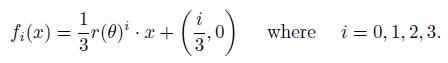
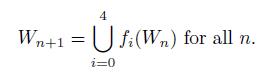
Here r(θ) is the rotation matrix with angle θ. We define the set {W n : n ∈ ℕ 0 } ⊆ ℝ2 inductively by,

We can define K = lim n→∞ W n with the limit in the Hausdorff metric. The set K is called the Kosh curve. In particular, W n approximates the Kosh curve where we construct discrete differential operators that are approximate to differential operators defined on the Kosh curve K.
Figure 1 The first four iterations of the construction off the Kosh curve: W 1 (Up right), W 2 (Up left), W 3 (down right), W 4 (down left).
● The Sierpinski triangle: The Sierpinski triangle is one of the most known examples of self-similar, see [4]. It can be consider a benchmark fractal where several ques-tions and problems can be test out. A construction of the triangle goes as follows. Let α
0 = (0, 0), α
1 = (1, 0), α
2 = (
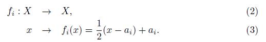
 ) the vertices of the equilateral triangle ⊆ ℝ2. We consider the set X with the Euclidean distance. For each i = 0, 1, 2 we define the affine mapping
Let W 0 = [α 0 , α 1] ∪ [α 1 , α 2] ∪ [α 2 , α 0] and we define {W n : n ∈ ℕ0 } by

As before, we see that K = W ∞ = lim n→∞ W n (where the limit is taken in the Hausdorff metric), and W n can be viewed as an approximation of K where differ-ential operators can be computed to approximation differential operators defined on K.
The Hata tree in the plane: W 0 = [p 1 , p 2]. Define
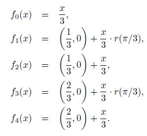
Figure 2 The first four iterations of the Sierpinski triangle: W 1 (up right), W 2 (up left), W 3 (up right), W 4 (up left).
Where r(θ) denotes the θ-rotation matrix. Define
The first four iterations are illustrated in Figure 3.
Figure 3 The first four iteration of the Hata tree W 1 (up right), W 2 (up left), W 3 (down right) and W 4 (down left).
Non-planar Hata tree: Let p 1 = (0, 0, 0) and p 2 = (0, 0, 1) the vertices of the set W 0 = [p 1 , p 2]. Define,
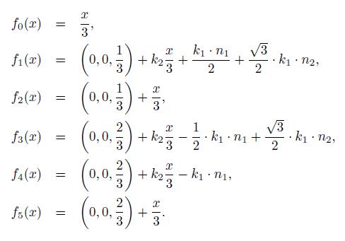
Where
 and
and
 is and orthonormal set.
Figure 4 The firstfour iteration of the Hata tree. See W 1 (Up right), W 2 (Up left), W 3 (Down right) and W 4 (Down Left).
The previous fractals can be built from the set of initial vertices V 0 and use the sequence V n+1 = f 1(V n ) ∪ ... ∪ f N (V n ). We will use this notation later on. For example, for the Sierpinski triangle the initial vertices are V0 = {α1, α 2, α 3} and we will have the sequence V n+1 = f 1(V n ) ∪ ... ∪ f 3(V n ), and Sierpinski triangle is V ∞ =∪∞ i=1 f i (V n ). From now on, the development of the theory will focus on the Sierpinski triangle.
3. Laplacian on a graph
In this section, we review the construction of the Laplace operator and the energy on a graph; in particular, we introduce the renormalization constant, which is important to get a finite limit of the energies associated with a family of graphs that approximates a fractal. See [5, 6, 9].
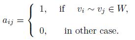
Let G(V, W ) a finite graph, where V = {v 1 , v 2 , ..., v n } determines the set of vertices and W the set of edge (without orientation) of V . If v, w ∈ V and exist an edge between v and w we write v ∼ w ∈ W. define the adjacency matrix A G associate to a graph G as the n × n matrix A G = [α ij ] i,j n =1, where
The weight matrix P G of G is the diagonal matrix of dimension n × n defined by P G = [p ij ] n i,j=1 with p ij = 0 when i # j and p ii is the number of adjacent vertices to v i , i = 1, . . . , n. Therefore,

The Laplacian matrix associate to G(V, W ) is given by
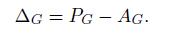
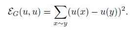
If u: V → ℝ we define the energy of u by
The bilinear form associated to the energy is
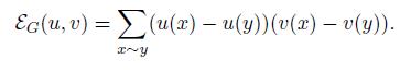
We denote ε(u) = ε (u, u). If we introduce the vectors ⃗
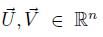 given by ⃗

 and ⃗
and ⃗
 , then

We observe that matrix ∆
G
is the matrix representation of the energy ε
G
. Now we consider the approximations
 to a fractal set K. We denote the energy associated to V
n
by
to a fractal set K. We denote the energy associated to V
n
by

The renormalized energy of level n = 2, 3, . . . can be computed for u n : V n → ℝ as

Here r n is a renormalization constant needed in order to obtain a non-increasing sequence of renormalized energies ε n , n = 0, 1, . . . . This step is necessary to obtain well-defined energy defined on K that we introduce as a limit of the renormalized energies above. For more details see [6] and references therein.
3.1. The case of the Sierpinski triangle K
For the Sierpinski triangle, see [3], we obtain that the energy for f:
 defined for n ∈ ℕ 0 by
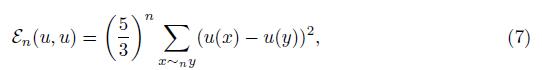
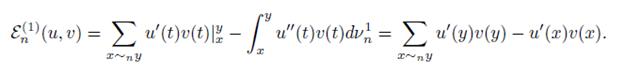
where x ∼ n y is the edge that connects to x with y and contained in W n . That is, the renormalization constant is r = (5/3). Then, we can compute ε(u, u) := lim n ε n (u| Vn , u| Vn ). Introduce the renormalized Laplace operators by
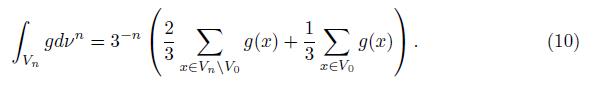
If we define the measure µ n on V n by assigning full measure 1 to V n and stating that each cell has the same measure (3 −n ), we see that we have
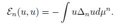
Using this it is defined the Laplace operator in K by
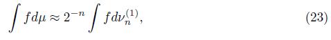
Here µ is the standard self-similar measure associated to K that can computed as the limit of the measure ν n in the sense that
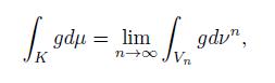
where we note that,
From here on, we will focus our study on the Sierpinski triangle.
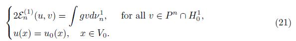
4. Formulations for the Dirichlet problem
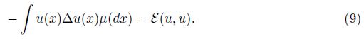
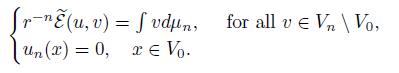
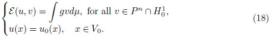
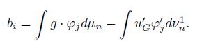
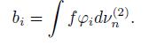
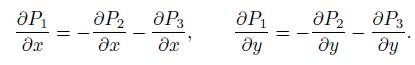
Given g: V ∞ → ℝ and u 0: V 0 → ℝ, we seek for u: V ∞ → ℝ such that
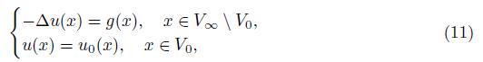
where ∆u(x) is defined in (9) and u 0 is the values of u in x ∈ V 0. We call this the strong formulation of the Dirichlet problem. Using the integration by parts formula we have
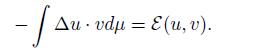
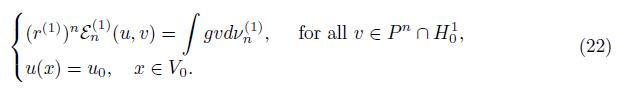
Therefore, we can write the problem as seeking for u with bounded energy, u ∈ H 1, such that
Here, H 1 = {u: V ∞ → ℝ, ε(v, v) < +∞} and H 0 1 = {v ∈ H 1: v(x) = 0, x ∈ V 0 }. We refer to these formulation as the weak form of the Dirichlet problem.
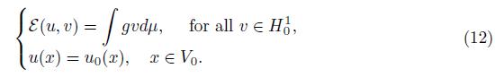
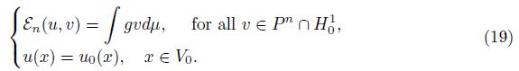
4.2. Finite difference approximation
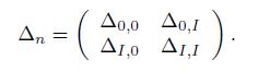
To approximate the solution of (11) in V n we consider ∆ n , the renormalized Laplace operator (defined for the Sierpinski triangle in (8)). Let the approximation be defined by u F D : V n → ℝ that can be written as u FD = {u F n D (x)} x∈Vn and we partitioned it as follows
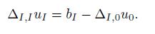
Note that u 0 is know and corresponds to the boundary values. Analogously for b FD = {g(x)} x∈Vn = [b 0 , b I ]. We obtain the block structure
We compute u I as the solution of
The main issue with this discrete formulation is that we need to know the renormalization constant: the value 5 n in the case of the Sierpinski triangle, see (8). The renormalization constant can be viewed as a scaling of the forcing term in the linear system. This scaling can be approximated as explained next.
4.3. Computation of the renormalization constant
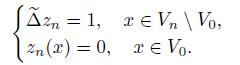
First we consider the finite difference method renormalization constant. The idea is to use the problem,
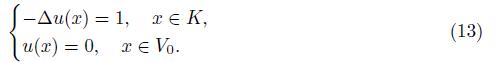
Denote by q n and approximation of the renormalization factor that we want to compute. The space of study is V n /V 0. We can approximate (13) by
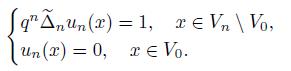
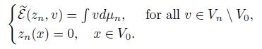
We want to compute the value q n . Numerically we can compute the solution of the problem, see [7],
We must have that z
n
(x) = q
n
u
n
(x), x ∈ V
n
since
 is nonsingular. For Vn+1 we will have z
n+1
= q
n+1
u
n+1
. Note that z
n
and z
n+1
can be calculated without knowing q
n
. For n large enough we should have,
is nonsingular. For Vn+1 we will have z
n+1
= q
n+1
u
n+1
. Note that z
n
and z
n+1
can be calculated without knowing q
n
. For n large enough we should have,
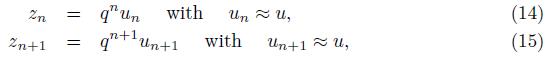
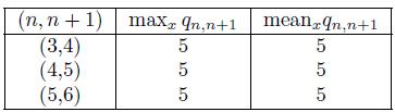
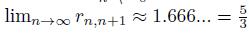
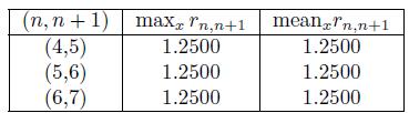
where u is the exact solution of (13). Therefore we should be able to use the approximation,
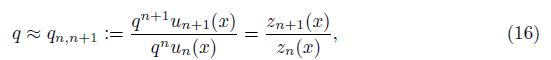
where x ∈ V n \V 0. See some numerical illustration in Table 1 for the case of the Sierpinski triangle. In this case we see hat lim n→∞ q n,n+1 = 5.
A similar procedure can be implemented for the energy renormalization constants. The weak form of (13) is written as,
Compute the solution of the graph energy problem (without renormalization),
We can then define the approximation,

Here x ∈ V
n
\ V
0. See a numerical verification in Table 2. In this case we should have
 .
.
4.4. Renormalized finite elements methods- rFEMs
Now we construct approximations for the weak form (12). That is, we propose approxi-mations for the computations of renormalized energy bilinear forms by rescaling standard approximations as introduced in Section 4.3.
We defined P n = {u: V n → ℝ}. We then project the weak formulation into the space P n . In the Galerkin formulation we seek to find u ∈ P n such that
Both u and v are defined on V n , then this formulation is equivalent to
We propose several classical finite element methods procedures in one and two dimensions to approximate the renormalized energy. Note that we can use the energy ε n rather than the limit ε. The renormalization constant is then computed by a procedure similar to the one explained previously. We recall that in this section we consider the case of the Sierpinski triangle.
Integrals along the edges
Recall that
 . Introduce the bilinear form,
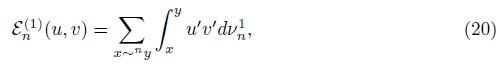
where u ′ denotes the one dimensional derivative along [x, y] of the linear interpolation of the vertex values u(x) and u(y). The measure ν n 1 is defined as the length measure along the edges of W n (rescaled to obtain total length 1). Note that for each n there are total 3 n+1 edges (3 for each cell). Each edge of V n has length 2 −n . Given a total length of 3(3/2) n before length rescaling.
We consider the following discrete problem,
As before we can write u = u I + u G where u G (x) = g(x), x ∈ V 0; u G (x) = 0, x ∈ V n \ V 0. Analogously u I ∈ P n tal such that u I (x) = 0 for x ∈ V 0. We then have,
This is equivalent to the linear system,
Let V n \ V 0 = {x 1 , x 2 , ..., x p } the set of interior vertices and we have,
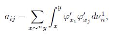
where φ xi is the linear interpolation of the characteristic functions of {x i } in V n . We also have
It is easy to see that
Recall that, on the left hand side above we use the piecewise liner interpolation of the nodal value of g. The previous formulation have to be renomarlized to
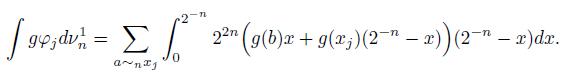
We note the following relation between the renormalized measure and the measure in-duced by the length measure, for any n, we have
that follows by computing the length integrals using the trapezoidal rule.
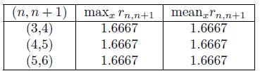
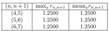
The renormalization constant r1 can be approximated using the procedure described in Section 4.3 by solving consecutive refinement level approximations with the constant function 1 as the right hand side and Dirichlet boundary conditions. See (17). In Table 3 we show the results of computing the renormalization constant.
In this case the renormalization constant can also be computed analytically. Integration by parts and the fact that we use piecewise linear interpolation (u ′′ = 0 inside edges) yields
Having into account that the length of the edges of the n approximation of K is 1/2 n , we get,

Therefor
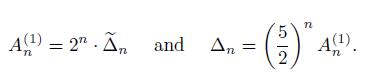
Due to (23) and (7) we see that renormalization constant for the family
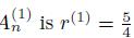 . In Table 3 we show the results of computing the renormalization constant using the procedure explained in Section 4.3. This a numerical verification that for the case of the Sierpinski triangle the computation agrees with the exact value of the renormalization constant just derived.
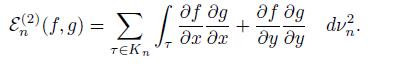
Area integrals
Introduce the bilinear form,
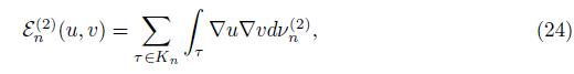
where ∇u denotes the two-dimensional gradient of the two-dimensional linear interpo-lation of the nodal value of u in the triangle τ. The measure ν
n
2 is the area measure restricted to Kn and normalized such that the total area of (all the triangles of) Vn is one. Note that, for each n, there is 3
n
each of them of área
 for a total area of
 before rescaling.
We formulate the following discrete problem,
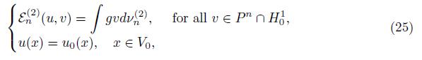
This time the previous formulation is equivalent to the linear system,
Where
and
As before, a renormalization is needed, that is,
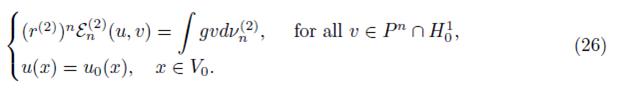
The renormalization constant r (2 can be approximated using the procedure described in Section 4.3 by solving consecutive refinement level approximations with the constant function 1 as the right hand side and Dirichlet boundary conditions. See (17). In Table 4 we show the results of computing the renormalization constant.
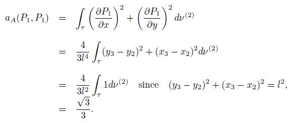
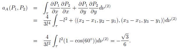
In order to verify our computations we compute the renormalization constant analytically. This is possible in this case. Recall that,
We use standard finite element analysis. Introduce the reference basis functions
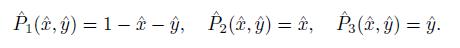
defined in the reference triangle 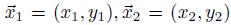 and ⃗
and ⃗

 , this mapping is given by F
τ
:
, this mapping is given by F
τ
:
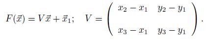
Define
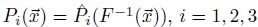 . Any linear function on τ is a linear combination of the basis functions P
1
, P
2
, P 3, in particular if u is a linear function on τ we have u(ψ) = u(x)P
1(ψ)+u(y)P
2(ψ)+u(z)P
3(ψ). From the definition of Pi is easy to see that
. Any linear function on τ is a linear combination of the basis functions P
1
, P
2
, P 3, in particular if u is a linear function on τ we have u(ψ) = u(x)P
1(ψ)+u(y)P
2(ψ)+u(z)P
3(ψ). From the definition of Pi is easy to see that
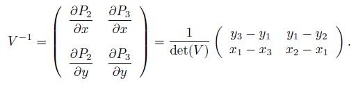
Moreover, we also have,
We also recall that det
 where l = 2-n then diameter of the triangle. We can compute
Analogously we have,
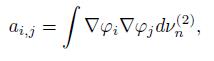
Having into account that each interior node belongs only to two-triangles and that two distinct nodes share an edge in at most one triangle, we conclude that the assembled global matrix is given by
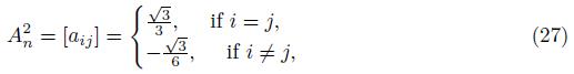
where i and j corresponds to the index of interior nodes. We see that,
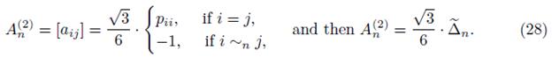
Recall that
We note the following relation between the renormalized measure and the measure in-duced by the area measure, for any n, we have
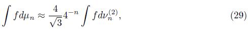
that follows by computing the length integrals using the trapezoidal rule.
From (28) and (29), we then have that the exact value of the renormalization constant is the same as the one for the construction based on length measures. This result verifies the numerical computations obtained in Table 4.
4.5. 4.5. Illustrations of the numerical methods
This section shows the numerical solution of the Laplace equation posed in some fractal sets. In particular, we consider the Sierpinski triangle, the Kosh curve, and two Hata trees. As we discussed before, we can approximate the solution by
▪ Renormalized Finite Difference (rFD):
Pre-processing: We solve a model problem with a given Dirichlet condition and g(x) = 1 as the forcing term in several graph approximations of the fractal set to compute an approximation of the renormalization constant.
Online step: we solve for the actual forcing term with the renormalized graph laplacian using the approximation of the renormalization constant computed in the pre-processing step.
▪ Renormalized Finite Element Method with line integrals (rFEM1D):
Pre-processing: approximation of the renormalization constant as before.
Online step: solution with actual right-hand side
▪ Renormalized Finite Element Method with area integrals (rFEM2D):
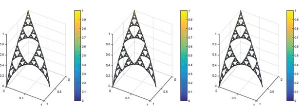
The Sierpinski triangle
For problems posed on the Sierpinski triangle recall that V 0 = {α 0 , α 1 , α 2 }. We want to approximate the solution of
In Figure 5 we illustrate some results.
The Kosh curve
For problems posed on the Kosh curve, recall that V 0 = {(0, 0), (1, 0)}. We want to approximate the solution of
We use the method introduced in section 4.4; if we associate the Laplacian with the energy defined by integrations over the edges, we have
where µ
n
is the length measure restricted to edges and
 was computed in Table (6) using the procedure described in Section 4.3.
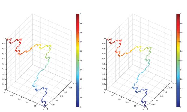
Figure 6 Approximated solution with rFD (left) and rFEM1D (right). Here g(x, y) = sin(x+y), u(α 0) = 1, u(α 1) = 0 and we consider V 5 the fifth level approximation of the Kosh curve.
The Hata tree
In the find method, the solution of the following equation is the same as that studied before, where V 0 = {(0, 0), (1, 0)}.
if we associate the Laplacian with the energy on edge, we have
Where µ
n
is the self-similar measure that the Kosh curve and the renormalization con-stant is given for
 , see Table 6.
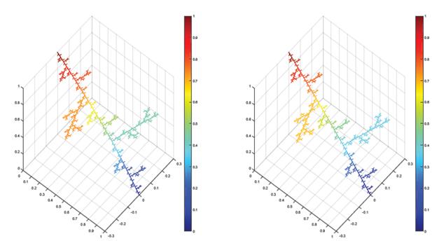
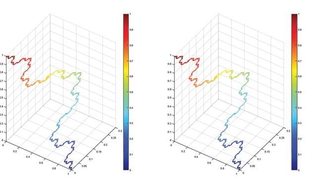
Figure 8 Approximated solution with rFD (left) and rFEM1D (right). Here g(x, y) = sin(x+y), u(α 0) = 1, u(α 1) = 0 and we consider V 3 the third level approximation of the Hata tree.
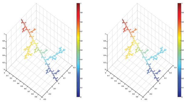
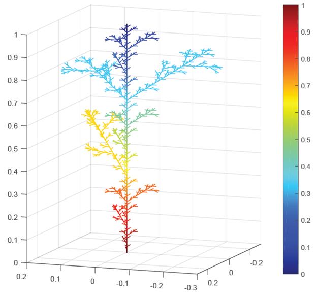
Hata tree in the space
For this fractal we use only rFD method (4.2), In Figure 10 we present a computed solution.
5. Conclusions
This paper designed a numerical procedure to approximate solutions to diffusion problems on self-similar fractal sets. We start with a discrete approximation of the fractal and the derivatives in standard non-renormalized formulations. We can then precompute the renormalization constant needed to approximate the actual differential operators on the fractal set. In particular, we present examples with the Sierpinski triangle using standard graph weights and adjacency matrices (Finite Difference method) or using week forms with length or area measures (Finite Element method). In the Finite Element method with the length measure, the derivatives in the weak forms are classical derivatives along the edges with integration concerning the length measure. In the finite element method with the area measure, we use partial derivatives with integration in two dimensions on triangles of the approximation of the Sierpinski triangle. We also present additional illustrations with the Kosh curve and the Hata tree.
It is also important to mention that the implementation of proposed finite element methods are simple and do not have significant changes with respect to the finite element method for differential equations in open domains. Also, the renormalization constant does not need to be known a priori. We can use finite element codes that work on tri-angulations in general, and only the “ triangulation” or graph that approximates the fractal must be used as input for these codes. The renormalization constant can be pre-computed as proposed in this paper. We observe that diffusion processes on these fractal sets can be approximated by classical diffusion processes (involving classical derivatives) on fractal approximations. These must be rescaled by the scale parameter that can be precomputed. The authors will explore this idea and the related numerical analysis in future works.

