The Price Setting Behavior in Colombia: Evidence from Micro Data

Juan Manuel Julio; Héctor Zárate

* The authors indebt very much the comments and helpful suggestions of Fernando Tenjo from the Board of Governors, Hernando Vargas, Deputy Governor, Andrés González, Chairman of the Macro Models Department, Edgar Caicedo, Munir Jalil and Javier Gómez from the bank’s staff. We are also grateful to the Statistics section of the Economic Research Vice presidency for their valuable assistance with the data set, all of them of the Banco de la República. However, any remaining errors as well as the results and opinions contained in this paper are the sole responsibility of its authors and do not compromise the Banco de la República, its Board of Governors or the Universidad Nacional de Colombia.

The autors are, in order, researcher of the Macroeconomic Models Department and Chief of Statistics Division, of the Banco de la República and proffesors in the Universidad Nacional de Colombia.

E-mails: jjulioro@banrep.gov.co, corresponding author, and hzaratso@banrep.gov.co

Document received; 25 January 2008; final version accepted: 31 March 2008.

* Agradecemos los valiosos comentarios de Fernando Tenjo de la Junta Directiva Hernando Vargas, gerente Técnico, Andrés González, director del Departamento de Modelos Macroeconómicos, Edgar Caicedo, Munir Jalil y Javier Gómez del equipo técnico. También agradecemos a la Sección de Estadística de la Subgerencia de Estudios Económicos por su colaboración con la base de datos, todos ellos del Banco de la República. Sin embargo, todos los errores, así como los resultados y opiniones que contiene este escrito son responsabilidad exclusiva de los autores y no comprometen al Banco de la República, su junta Directiva o a la Universidad Nacional de Colombia.

In this paper we explore the price setting behavior of Colombian producers and importers using a unique database containing the monthly price reports underlying the Colombian PPI from Jun-1999 to Oct-2006. We focus on five particular questions: 1. Are prices sticky or flexible? 2. Is a price increase more likely than a decrease? 3. Are price changes synchronized? 4. Is the pricing rule state or time dependent? 5. Are price changes sizable? Answers to these questions provide some of the micro fundamentals for the design of monetary policy in this country.

Key Words: Price Setting Behavior, Sticky Prices, PPI JEL Classification: E31, E52, E58

Usando una base de datos única que contiene los reportes de precios utilizados para el cómputo del índice de precios al productor (IPP) desde junio de 1999 hasta octubre de 2006, en este trabajo exploramos la manera como los productores e importadores colombianos fijan sus precios. Nos enfocamos en cinco preguntas, a saber: 1) ¿son los precios rígidos o flexibles? 2) ¿Es más probable un incremento que una disminución de precios? 3) ¿Están sincronizados los cambios de los precios? 4) ¿La regla de fijación de precios es dependiente de factores de estado o de tiempo? 5) ¿Son grandes las actualizaciones de los precios? Las respuestas a estas preguntas proveen la microfundamentación para el diseño de la política monetaria en este país.

Palabras clave: Fijación de los precios, rigideces de precios, IPP.

Clasificación JEL: E31, E52, E58.

Usando uma base de dados única, a qual contém os reportes de preços utilizados para o cômputo do índice de preços do produtor (IPP) desde junho de 1999 até outubro de 2006, neste trabalho exploramos a maneira como os produtores e importadores colombianos fixam os seus preços. Nos enfocamos em cinco perguntas, a saber: 1) são os preços rígidos ou flexíveis?; 2) é mais provável um incremento que uma diminuição de preços?; 3) estão sincronizadas as mudanças dos preços?; 4) a regra de fixação de preços dependem de fatores de estado ou de tempo?, e 5) são grandes as atualizações dos preços? As respostas a estas perguntas provêem a micro-fundamentação para o desenho da política monetária neste país.

Palavras chave: fixação dos preços, rigidezes de preços, índice de preços do produtor (IPP).

Classificação JEL: E31, E52, E58.

1. Introduction

The assumption that prices are sticky has become an important factor in the design of monetary policy models. In fact, theoretical studies have shown that the degree of price flexibility has an important effect on the response of key variables to economic innovations¹. Therefore, price stickiness is an important source of short to medium term non neutrality in monetary policy models. See Bils and Klenow (2004), Taylor (1980) and Rothemberg (1982).

More precisely, the degree of price flexibility determines the slope of the new Keynesian Phillips curve, which implies that the dynamic behavior of the inflation rate, in response to marginal costs innovations, is highly dependent on the pricing rule used in the model. Thus, price stickiness has an important effect on the degree of inflation (as well as many other variables) persistence, a key determinant of monetary policy. Thus, price stickiness has also an important effect on the design of monetary policies² (see Angeloni et al., 2006).

Acknowledging the importance of price stickiness, inflation targeting central banks devote a great effort to study the features and determinants of the individual pricing rules that determine it. These features and determinants, in turn, provide the required micro foundations for monetary policy models.

Evidence on the price setting behavior in particular economies comes from two sources: Quantitative studies on individual price databases and firm’s surveys on qualitative pricing practices. Quantitative studies are particularly suited to study the price setting behavior since they contain a huge number of price quotes over a long time span. However, this evidence is usually complemented with surveys on qualitative features that might not be found otherwise³ (see Álvarez et al., 2005a).

There are several reasons to study the price setting behavior at the firm level. First, even though the final goal of the central bank is CPI inflation, several theories on the price setting behavior refer to producers rather than consumers prices. Second, theoretical studies have shown that a monetary policy that does not take into account PPI inflation, or PPI sector shocks, tends to produce larger welfare losses than a policy that targets CPI and PPI inflations (Huang and Liu, 2005). And third, monetary policy channels may differ, and be relatively more important, for producer prices than consumer prices, especially if the retail sector uses simple pricing rules (see Gautier, 2006, and Basu, 1995).

Furthermore, producer prices differ from consumers because producers have closer links with their costumers, which translate into long term relationships based on explicit contracts. Furthermore the lack of anonymity in producer markets leads to costumer resistance and, depending on the degree of competitiveness in the sector, increases the odds of collusion. In addition, costumer hierarchy is more important in producer markets, and price adjustment costs seem to be of less importance.

There are several alternative ways to set up pricing rules in monetary policy models. Pricing rules may be “time dependent” or “state dependent”. In time dependent rules, prices are kept constant for an exogenously determined random number of periods (Taylor contracts), or, an exogenously determined random fraction of firms is allowed to adjust prices to new information (Calvo rule). In state dependent rules the probability of a price change is endogenous to the state of the economy, but firms face costs related to the price change.

Price stickiness may be set up in several ways. For instance, the lack of price change synchronization has been identified as one of the main sources of price stickiness. In fact, producers seem to prefer slow price changes, to avoid large relative price movements, in the face of unsynchronized nominal innovations. In time dependent rules, for instance, price changes are not synchronized, and this lack of synchronization causes price inertia (see Blanchard, 1982).

Another way to introduce price stickiness in monetary policy models is by fixing differing degrees of inertia depending on the direction of the shock. In fact, it has been argued that prices are downward rigid. Some authors say that the price signals the quality of the good, and thus producers tend to avoid price reductions. Other authors propose that price reductions are rare because consumers do not respond as efficiently to reductions than to increases. Finally, some others suggest that, in the face of unsynchronized innovations, the strategic behavior of firms lead to downward rigidity.

The existence of strong downward rigidities relates to big welfare loses associated to monetary policy. However, a little downward rigidity, accompanied by a low inflation, ‘greases the wheels’ and allow real (i.e. relative) prices to fall when necessary for a stable long run inflation target.

Finally, some researchers propose that the cost of changing prices is an important source of price stickiness. In fact, if the cost curve is convex, with respect to the price change size, firms will avoid big price changes. In state dependent rules, for instance, price change costs are one the main sources of price stickiness.

In this paper we explore the price setting behavior of Colombian producers using the monthly price reports underlying the Colombian PPI from Jun-1999 to Oct-2006. Following our previous discussion, we focus on five particular questions: 1. Are prices sticky or flexible? 2. Is a price increase more likely than a decrease? 3. Are price changes synchronized? 4. Is the pricing rule state dependent or time dependent? 5. Are price changes sizable? Answers to these questions provide the micro economic foundations for the design of the monetary policy model in this country.

Being an exploratory work, we include little external information, and consequently, our results are mostly descriptive and unconditional. However, we interpret, as far as possible, our findings in terms of the possible models and macroeconomic implications.

Apart from the introduction, the paper is distributed as follows: in section two we describe the definitions we will use along the paper, which are common to price stickiness studies, we describe the dataset and its treatment (as it has an important effect on the results), we describe the methodology and the PPI’s weighing scheme. By describing the PPI’s weighing scheme, we propose a ranking according to the manufacture stage of goods, for an aggregated basket, that will be used to interpret the results of section three. In the fourth we conclude.

II. Methodology

A. Basic definitions

A particular product is a unique physical item or service that is traded in the economy, which has a clearly defined source (produced-and-consumed or imported), brand, presentation, packaging, unit of measure, and content, among others. A product category is a particular product whose price is reported by a clearly identified producer.

A product class is a basket or group of individual products. There are several ways to aggregate individual products in PPI databases. For the Colombian case, product classes or baskets refer to interactions, at different levels, of the source (produced-and-consumed or imported), the nine digits local adaptation of the CIIU code, and the destination (intermediate consumption, final consumption, capital goods and construction materials) of goods. Moreover, according to Banco de la República (1999), the PPI can be obtained according to many other alternative baskets.

The workhorse of price stickiness studies is the duration, that is, the length of time that the price of a product category remains constant. We also define a price sequence as an uninterrupted sequence of price reports belonging to a particular product category.

A particular product category might be associated to more than one price sequence due to the eventual appearance of missing values. Missing values may arise due to several reasons like the temporary unavailability of the informant, or the product category in a particular informant. In this case, PPI administrators follow very strict rules to impute missing values, like carrying over the last observed price or price change. On the other hand, when the informant or product unavailability is permanent, we refer to product or sample attrition.

A price spell is an uninterrupted sequence of constant price reports associated with a unique product category. As an example, Graph 1 presents five price sequences belonging to the same individual product, measured in five different cities. From this figure it can be observed that prices tend to move together in the long run, and that some sequences tend to provide longer spells than others. It is also observed that price changes lack synchronization. Finally, it should be noticed that big price changes are frequent as well as price reductions.

In most cases the beginning of the price sequence does not match the date a particular product category appears for the first time in the economy, thus the first spell is usually censored. In a similar way, the end of the last spell in a particular sequence might not match the disappearance of the particular product category, and therefore might be truncated. Truncation may arise because of involuntary product or informant attrition or voluntary attrition due to sample maintenance (see Baudri et al., 2004).

For a particular product category and price spell (s), price stickiness can be studied through the duration of the spell (Ts), or the frequency of price changes (Fs). The frequency of price changes is the fraction of the basket weight, belonging to a particular product class that changes their prices on a given period of time.

The duration (a time series measure) and frequency of price changes (across section measure), computed for the whole sample, relate to each other according to the formula:

from which an indirect non parametric duration estimate may be obtained.

Direct non parametric duration estimates rely on very few assumptions but require that all price spells to be non-censored. Indirect non parametric estimates, those derived from the frequency of price changes, can handle censored spells at the cost of assuming a constant hazard rate function⁴.

In Taylor contracts, for instance, the implied hazard function is generally increasing, depending on the duration distribution assumed. In state dependent rules the hazard function depends on the distribution of the innovations, and is usually increasing. A constant hazard function, like that implied in a deterministic Calvo pricing, is hard to justify in practice.

B. The data set

Our data set consists of 540,069 monthly list price reports collected from June 1999 to October 2006 in order to compute the Colombian PPI, excluding exports. On average there were 6,178 reports each month, which corresponds to the number of different product categories surveyed. The sampling and PPI computation methodology is described in Banco de la República (1999).

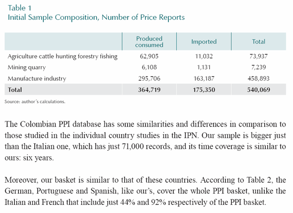
Imports make 32.5% of total PPI records and are concentrated in manufactures. Table 1 describes the composition of the initial sample according to its source (produced-and-consumed and imports) and the CIIU1 classification. Produced-and-consumed records make 67.5% of the sample, 85.1% of agriculture-cattle…,84.4% of mining-and-quarry and just 64.4% of manufactures.

The Colombian PPI database has some similarities and differences in comparison to those studied in the individual country studies in the IPN. Our sample is bigger just than the Italian one, which has just 71,000 records, and its time coverage is similar to ours: six years.

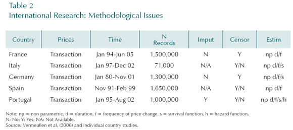
Moreover, our basket is similar to that of these countries. According to Table 2, the German, Portuguese and Spanish, like our’s, cover the whole PPI basket, unlike the Italian and French that include just 44% and 92% respectively of the PPI basket.

A unique feature of our database is that price reports are requested and recorded (i.e. ex post), when the reporter is temporarily unavailable. Certainly, these reports can not be used for PPI computation, but whenever ex post prices are observed they replace the corresponding missing or imputed values in our analysis. Imputation is performed for only three months, when the sample attrition is recorded.

Imputation is performed by carrying over the last observed price in its currency, and the currency value is updated at every period of time. The original sample contains 32,693 reports imputed by the PPI administrator, 6.10% of the original sample. However, there were still 1,750 missing values disconnecting some of the price sequences identified. These missing values were imputed, which gives a total of 34,443 imputed reports, 6.43% of the original sample.

Regarding imputation we follow the lead of the IPN individual country studies where all but the French and German studies report the use some kind of imputation (Table 2).

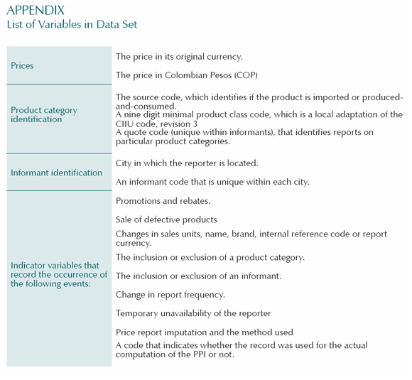
Our database contains indicator variables for the following events: sales, promotions, rebates, sale of defective products and sale of products by companies in the liquidation process. These reports were excluded from both our analysis and the PPI computation⁵. Altogether there were 3,768 reports deleted because of these events, 0.74% of the sample (see Appendix).

As far as taxes go, according to Banco de la República (1999), PPI prices are requested before taxes.

Finally, for most product categories prices are reported on a monthly basis. However, some informants schedule price changes at lower frequencies like quarters, semesters or years. Under these circumstances, the PPI survey is performed at the requested frequency, and the questionnaire continuously asks for frequency updates. Frequency changes are recorded in the database and the survey frequency is updated accordingly.

C. Weighing

The Colombian PPI has two levels of operating weights. At the highest disaggregation levels, such as the minimal classes and product categories, there is a flexible weighing scheme, which applies mostly to agricultural products. From there, CIIU7 and up, a fixed weighing scheme applies. For our estimates we use average weights when required.

We hypothesize that the pricing behavior of firms differ according to the source of goods (imports or produced-consumed), and its manufacture stage. The first is explained by both, the effect of exchange rate variations on the price of imports, and the type of innovations an importer is subject to, in comparison to a producer of locally consumed goods. The second relates to the fact that whenever unsynchronized innovations occur, firms prefer slow price adjustments, in order to avoid large relative price movements (see Blanchard, 1982, and Clark, 1999).

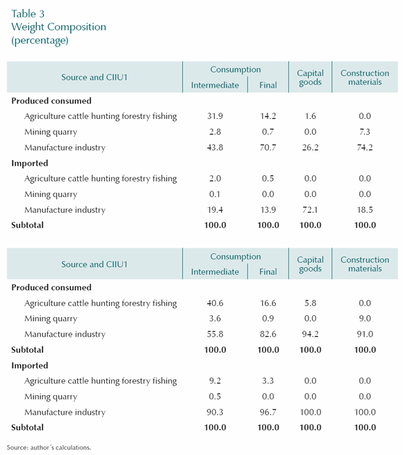
Table 3 shows the weight allocation, within each destination, according to the source (one digit CIIU code interaction). The organization of the table aims to emphasize both, the link between the destination of goods and their manufacture stage, proxied by the CIIU code, within each source, and the difference between imported and produced-consumed goods.

In the panel A of Table 3 destination weight shares add up 100% regardless of the source of goods, and in the panel B destination share weights add up 100% for each source⁶.

The panel A of Table 3 reveals that construction materials, intermediate and final consumption goods are dominated by produced-consumed goods. In fact, the shares of produced-consumed goods are 81.5%, 78% and 85.6% respectively and just 27.8% for capital goods. In addition, it should be noticed that imports are basically manufactures with a very small share of agriculture and mining.

The panel B of Table 3 reveals a more interesting picture. Destination, for produced-consumed goods at least, may be ranked according to the manufacture stage of goods. The ranking may be performed by comparing the share of agricultural and manufactures between them. In fact, for produced-consumed goods, the lowest share of manufactures (56%), and the highest of agriculture (41%), corresponds to intermediate consumption goods, setting this destination in the lowest manufacture stage level. The third is final consumption with 83% and 17% respectively. The second is capital goods with 94% and 6% respectively, and the first is construction goods, 91% manufactures and 9% mining and quarry, since the later have a higher manufacture stage than agricultural products.

This ordering will play an important role for the interpretation of results. However, for imports it is not possible to establish a similar ordering since the behavior of import prices is highly influenced by the import frequency.

D. Methodology

Direct estimation of the mean duration at any level of aggregation is based on non censored spells, that is, discarding the first and last spells of each price sequence. However, indirect duration estimates, derived from the frequency of price changes, include censored spells and thus might be more efficient and unbiased.

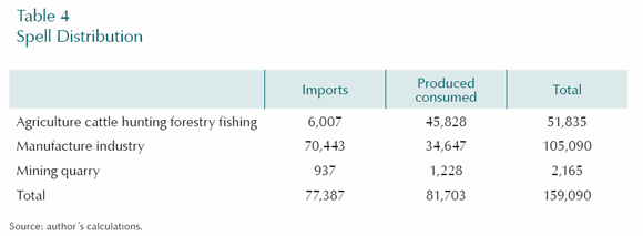
After discarding the first and last spells of every price sequence, there were 159,090 price spells remaining in the database, an average of 14.5 spells per sequence (Table 4).

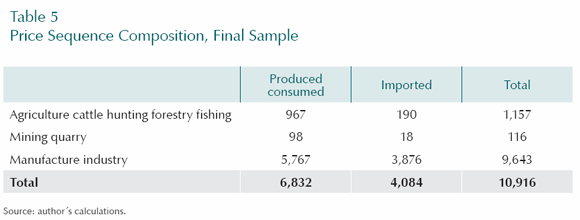
The price sequence composition according to the source and CIIU1 class they belong is similar to the record composition of the initial sample (Table 5).

Since our price sequences are not interrupted, each of them may be uniquely identified as a sequence of price reports P_mjkt⁹, where t=1,2,3,...,T is the time; k=1,2,3,...,K_mj identifies the product category reported by the j=1,2,3,...,Jm informant belonging to the m=1,2,3,...,M minimal class. The triplet (m, j, k) identifies a price sequence uniquely.

Let i=1,2,3,...,Nmjk be the identifier of the i – th price spell in the (m, j, k) sequence, and let T_mjkt be the i – th price spell duration. All the information regarding the i – th price spell can be summarized in the triplet (m, j, k), the price level, the spell’s starting date and duration.

We can estimate the mean duration for the (m, j, k) product category as

Since our database does not distinguish particular products, we can not compute any statistics at this level. Instead, we compute the average weighted duration for each minimal product class as

where α_jk is the average weight for each product category in the minimal product class.

Once we have estimated the average duration for each minimal product class, we can estimate the duration for wider aggregations by computing weighted averages using the corresponding average or fixed PPI weights.

where α_m is the PPI weight associated with the m – th minimal product class.

Given that we are unable to identify individual products, our aggregation starts with the minimal classes rather than individual products. This procedure affects the interpretation of our estimates at the minimal class level since these are, for the majority of the sample, unweighed averages of the product categories belonging to the minimal classes. However, no aggregation bias is expected to happen since the duration of price spells are computed for uniquely determined sequences.

Following the same procedure we can compute any statistic to characterize the distribution of durations. We focus on the median, the quartiles and standard deviation.

Indirect mean duration estimates may be obtained from the estimated mean frequency of price changes (FPC). The mean FPC is the average percentage of the basket changing its prices on a given period of time, and thus it is across sectional measure⁷ .

Indirect duration estimates require the computation of the frequency of price changes for each product category, thus, we define a binary variable indicating a price change

and then, the estimated FPC for the m-th minimal class at time t can be computed as

and

Following the same procedure we compute the frequency of price increases and decreases.

III. How Colombian Producer’s Change Their Prices?

A. Are sticky flexible?

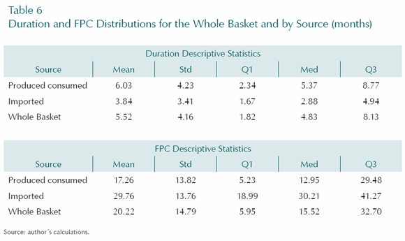
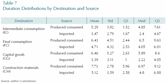
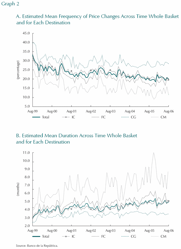
To answer this question, the estimated duration and frequency of price changes (FPC), distributions are studied for increasingly disaggregated baskets up to the minimal classes. Distributions according to the destination and source of goods are also studied. The results are shown in tables 6 and 7 as well as in Graph2, panels A and B. Further breakdowns are available from the authors.

Findings about this issue summarize in the following points.

- The average weighed duration of producer’s prices is 5.52 months, 20.2% of the basket change it prices each month, but there is a sizable degree of duration heterogeneity between and within product classes. The weighed standard deviation of durations is 4.16 months (Table 6).

- Heterogeneity might be explained in part by the source of goods. Because of COP/USD exchange rate variation, not only there is a sharp difference in average duration, 3.84 months for imported and 6.03 for produced-and-consumed, but there are also homogeneity gains within imported goods as its weighed standard deviation reduces to 3.41 months, and the coefficient of variation for produced-and-consumed reduces with respect to that of the total basket (Table 6).

- Price duration heterogeneity might also be explained by the manufacture stage of goods. For produced-and-consumed goods, duration ranking is similar to the one obtained by analyzing the PPI weighing structure in section II.3. Construction materials have the largest duration (7.73 months), intermediate consumption the lowest (5.29) and final consumption and capital goods are in the middle (6.43 and 6.46 months, respectively). There are also clear homogeneity gains as the intermediate consumption and construction materials standard deviation (3.92 and 2.78 months, respectively), are smaller than those of the total produced-and-consumed basket (4.23 months). Surprisingly, the coefficient of variation of construction materials reduces to 2.78 showing a striking heterogeneity reduction for this basket (tables 6 and 7).

- Estimated duration increases as the inflation rate decreases. In fact, setting aside basket differences, our findings are consistent with Colombian CPI results. Jaramillo and Cerquera (1999) concluded that, on average, consumer prices remained constant for two months during a period of moderately high average CPI inflation of 28%. Espinosa, Jaramillo and Caicedo (2001) found a mean duration of four months during a period when the average CPI inflation rate was 25%, and our results show an estimated mean duration of 5.5 months in a period when the producers price inflation is 7%. Moreover, Graph 2B show a clear upward duration trend with a higher slope during 1999 and 2000, as expected from the rapid inflation adjustment after the 1998 crises. Afterwards the trend is small but steady, consistent with the steady small downward trend the inflation rate has followed since 2000.

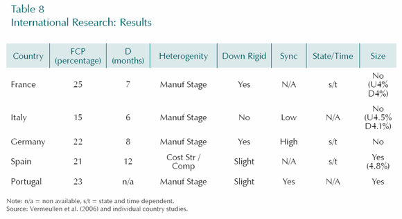
- The analysis of the FPC distribution leads to similar results. Colombian outcomes are analogous to those of the IPN. The weighted average FPC for the whole euro-area is 21%. The highest flexibility is found for France, where 25% of producer prices change each month, and the highest stickiness for Italy, where 15% of producer prices change every month, on average. Colombian results, 20% each month, lie in a middle range. However, if we take into account that the inflation rate during the sample for the countries of the IPN was lower than 2.5% and the Colombian was 7%, this evidence suggests that Colombian prices are stickier than those of the IPN (see Vermeullen et al., 2007) (Table 8).

More interestingly, individual country studies, as well as the EU summaries, report a high degree of duration heterogeneity within and between product classes. Vermeullen et al. (2007), reports that individual country data bases in the EU consistently point to a direct relationship between duration of producer price spells and the amount of transformation required to produce the particular items. See Table 8 also.

These results, Colombian as well IPN, agree with Blanchard (1982), who proposes that price setting must be influenced by the number of manufacturing stages. This author argues that, “Desynchronization implies snake effects, i.e. movements in factor prices slowly transmitted to intermediate and final good prices (pp. 2).” Thus, stickiness relate directly to the number of production steps required by the particular good. Therefore, goods lower in the manufacture stage scale have higher price and profit variability than those high up in this scale.

B. Is a price increase more likely than decrease?

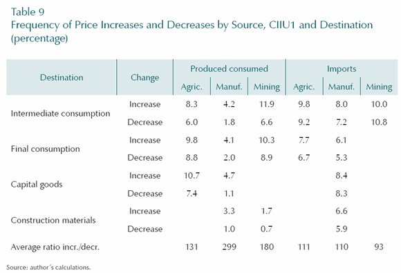
In order to answer this question, we compute the average frequency of price increases and decreases according to the source, destination and CIIU1 classification code of goods. Results are presented in Table 9 and the corresponding findings summarize in the following points:

- Price increases are slightly more likely to happen than decreases. In fact, only in one case, mining imports destined to intermediate consumption, the frequency of price increases is lower than that of decreases, 10% and 10.8% respectively (Table 9).

- The ratio between the frequency of price increases and decreases is higher for produced-and-consumed goods in comparison to imported ones. In just one case, agricultural products destined to final consumption, it is higher for imports. Thus, there is a clear difference in the behavior of price increases over decreases between sources of goods (Table 9).

- The ratio between the frequency of price increases and decreases relates to the manufacture stage of goods too. Within produced-consumed goods, the average ratio is highest for manufactures, middle for mining and lowest for agriculture. A similar order is observed for imports if we take into account that agricultural imports in Colombia correspond chiefly to highly processed foods (Table 8).

- There is a surprisingly high frequency of price decreases. Finding a slight downward nominal rigidity in producer prices is not surprising, given that a positive inflation of moderate size was observed in the sample span for Colombia. Moreover, this slight downward rigidity justifies the choice of a 3% long run inflation target in Colombia, since it permits that real (relative) prices reduce when required to maintain the long term objective. Moreover, the finding of no strong downward rigidities, in comparison to the six IPN countries, indicates that the welfare costs of monetary policy due to this kind of stickiness are not bigger than in the EU. See Table 8.

C. Are price changes synchronized within minimal classes?

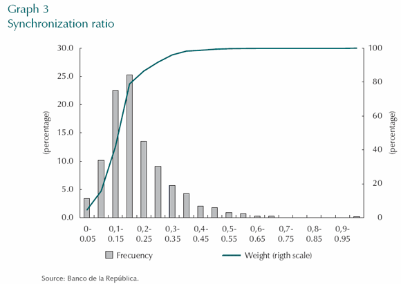
In order to determine the degree of synchronization of product changes, we compute a synchronization measure proposed by Fisher and Konieczni (2000). Under the assumption of perfect synchronization, these authors propose to use the ratio between the standard deviation of the monthly frequencies of price changes at the minimal class level, and the theoretical standard deviation implied by the average frequency of price changes computed at the minimal class level that would be observed under the assumption of perfect synchronization. This ratio is one in the case of perfect synchronization and zero with perfect staggering⁸ (see, also, Aucremane and Dhyne, 2004, and Díaz, 2004).

The results are presented in graph2 and 3 and the main finding comprise in the following point.

This finding is consistent with the view that the lack of synchronization yields price stickiness. In fact, Italian researchers find strong evidence of staggering (in agreement with its high stickiness), and German researchers find evidence of a high degree of synchronization in particular industrial sectors (which agrees with its low stickiness). Therefore, the Colombian price stickiness seems to be related to a low synchronization level. See Table 8.

D. Is the pricing rule “state dependent” or “time dependent”?

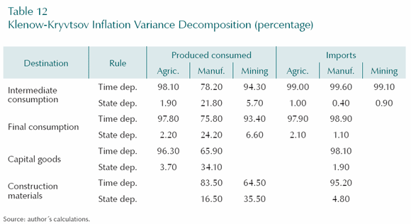
In order to answer this question, we present two types of evidence; a conditional logistic model and the Klenow and Kryvtsov (2003) inflation variance decomposition⁹. The first helps determine the factors affecting the choice of changing or not producer prices. The second helps asses the importance of time dependence and state dependence in producer’s pricings rules.

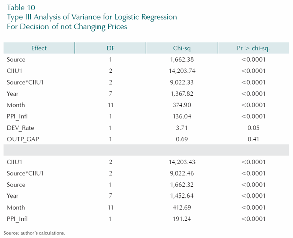
The conditional logistic model explains the probability of no price change at the product category level. The explanatory variables, according to the previous discussions, are the source code, source, the CIIU1 code, the year and month of the price report, the monthly devaluation rate, the inflation rate and the output gap. Since our logistic analysis involves some categorical factors, CIIU1, the year and month of the report, the overall factor significance is studied through the type III analysis of variance. Table 10 contains this analysis for the model including all the regressors (upper panel), and the factors remaining after a stepwise factor selection procedure in the lower panel.

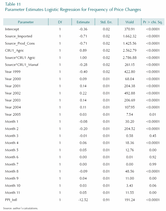
The results are presented in tables 10 to 12, and the findings summarize in the following points:

- There is clear presence of time and state dependence in producer’s pricing rules, but time dependence dominate. In fact, time related variables like the month and year of the report are clearly more significant than those related to the state of the economy in the conditional logistic model. Moreover, due to the correlation between the inflation rate and the output gap, only the inflation rate enters into the model (see Table 10, bottom panel). However, after removing the inflation rate, the output gap significance improves greatly. These findings are confirmed in Table 11, where the final model estimates are presented, and in Table 12 where the Klenow and Kryvtsov decomposition is shown. From Table 12 it can be observed that consistently the time dependency contribution to the inflation variance is substantially bigger, in all categories and classifications, than the state contribution.

In addition, it should be noted that, in agreement with our previous discussion, the source and manufacture state of goods (CIIU1), as well as their interaction, are the most important factors explaining the decision of changing prices.

- For produced-and-consumed goods state dependency seems to relate to the manufacture stage of goods. In fact, the state dependence contribution is higher, between 16.5% and 34%, for produced-consumed manufactures regardless of their destination.

International studies also find evidence of strong time dependency in producer prices with a small but significant contribution of state dependency. In the case of France, for instance, the average time dependence contribution is 92.2%. Strong time dependency in producer prices may arise because of the higher reliance on explicit contracts and costumer resistance. See Table 8.

E. Are price changes sizable?

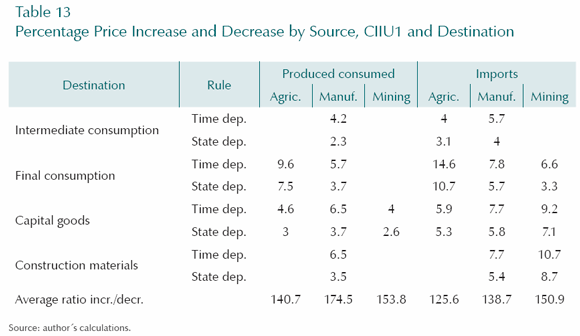
In order to answer this question, the weighted average percentage price increase and decrease were computed. The results are contained in Table 13 and the findings summarize in the following points.

- Percentage price increases and decreases are not sizably different from the average inflation level during the sample span (Table 13).

- However, this evidence implies that a big amount of the basket changing its prices above the inflation, in absolute value. That is, price changes bigger than the inflation rate in absolute value, are frequent. This evidence suggests that costs are not convex (Table 13).

- Percentage price increase and decrease heterogeneity has to do with the source of goods. Percentage price increases and decreases are uniformly lower for imported goods than produced-consumed goods.

- Percentage price increase and decrease heterogeneity has to do with the manufacture stage of goods. For produced-consumed goods, the average ratio of increases over decreases is smallest for agriculture, 140.7%, second for mining, 153.8% and highest for manufactures, 174.5%. A similar ordering is found for imports. International evidence on the existence of convex costs agrees with our findings (see Vermeullen, et al., 2007) and Table 8.

IV. Conclusion

Colombian producers and importers change their prices relatively frequently: 20.2% of the basket each month. Although this result is similar to those of the six countries of the IPN, taking into account the inflation rate prevailing during the sample, our prices are stickier than theirs. This result implies that, ceteris paribus, our cycles are deeper than those of the EU.

Looking for an explanation to this level of stickiness, we found that the lack of synchronization seems to be a very important factor. However, the costs of price changes do not seem to be convex. Therefore, the costs of price changes do not seem to matter much when firms decide a price change.

However, we found some evidence of seasonal synchronization that may be related to the minimum wage increase schedule and explicit contracts. Nevertheless, a surprisingly high frequency of price decreases of moderate size was found given the level of PPI inflation prevailing during the sample.

In addition, a slight nominal downward rigidity was found. This downward rigidity relate to the efficiency of the price system, as it permits to set a long run inflation target of 3%.

However, no signs of strong nominal downward rigidities were found. Therefore, the high welfare costs of monetary policy related to strong nominal rigidities, at least in comparison to the countries in the IPN, are ruled out for Colombia.

Moreover, we found that the decision to change prices is determined by both, state and time dependent factors, dominated by the later. That is, like in Taylor contracts.

Also strong sectoral differences in the price setting behavior of firms were found. These sectoral differences relate to the source and manufacture stage of goods. In fact, import prices are more flexible, both in absolute and downward terms, than produced-and-consumed ones. Moreover, produced-and-consumed goods are stickier, both in absolute and downward, as their manufacture stage increases. In addition, the state dependence component is higher for produced-and-consumed goods than for the rest of the basket.

Consequently, imports and low manufactured goods respond quicker to monetary policy than those higher up in the manufacture stage scale.

Finally, setting aside basket differences, our findings are consistent with previous results. Jaramillo and Cerquera (1999) concluded that, on average, consumer prices remained constant for two months during a period when the average CPI inflation was 28%. Espinosa, Jaramillo and Caicedo (2001), estimated a mean duration of four months during a period when the average CPI inflation rate was 25%. Our results show an estimate of 5.5 months during a period when the producers price inflation was 7%.

This fact, according to Angeloni et al. (2006), implies that the sensibility of the overall inflation persistence to cost push and demand shocks as well as past inflation reduced along with the inflation rate. Therefore, a direct relationship between inflation and persistence is implied, ceteris paribus. This prediction, according to Taylor (2000), implies that the reduction of the inflation rate, derived from the increase in credibility during the 1990s, reduced the pricing power of firms, which in turn helped keep a downward inflation trend. However, according to Taylor’s predictions, these benefits (decreasing inflation and increasing growth), “can disappear if monetary policy and expectations change” p. 2.

Comments

¹Price stickiness relate to the fact that the price of goods and services do not react immediately to demand or supply innovations.

² Inflation persistence has to do with the dynamic behavior of the inflation rate (with respect to an “equilibrium”), after the economy has been hit by a shock.

³ Given that firm surveys are performed on a low frequency basis, and in periods of time whose economic conditions rarely repeat in the future, they tend to focus on qualitative invariant price setting features like the type of information used to decide on price changes, the market power of firms, and so on.

⁴ The hazard function describes the probability of a price change conditional on no price change during the last k periods, as a function of k. The survival function is analogous to the hazard and determines the probability that a price spell lasts more than k periods.

⁵ Deleting the records corresponding to sales and rebates is a normal practice in price duration studies since they might reveal end of season, liquidating or other events not related to normal price strategies. However, their deletion might cause an upward duration bias since the related spells tend to be shorter than average. Since in our study these records are a very small percentage of the total sample its effect is expected to be negligible.

⁶ The whole weighing structure may be recovered from Table 3 by noticing that 38.8% of the PPI excluding exports corresponds to final consumption, 43.0% to intermediate consumption, 10.2% to capital goods and the remaining 8.0 % to construction goods.

⁷Non parametric indirect duration estimates derived from FPC’s assume the existence of a constant hazard function.

⁸For a given minimal class let pt be the mean FPC at t. The synchronization index proposed by Fisher and Konieczni may be computed as

⁹According to Klenow and Krivtsov the inflation rate might be decomposed as the product of the FPC and the percentage price change as E where P_t is the price level and D is the difference operator. The volatility of the first term figures prominently in many state dependent models, and the volatility of the second is the only source of fluctuations in time dependent pricing models. By writing E an exact variance decomposition is found, E where Cov_f=E. In the variance decomposition equation the first term is time dependent and the remaining two are the state dependent ones.

1. Altissimo, F.; Ehrmann, M.; Smets, F. “Inflation Persistence and Price Setting Behavior in the Euro-area, a Summary of the IPN Evidence”, working paper, no. 46, European Central Bank, 2006.        [ Links ]

2. Álvarez, L.; Buriel, P.; Hernando, I. “Do Decreasing Hazard Functions for Price Changes Make Sense”, working paper, no. 461, European Central Bank, 2005.        [ Links ]

3. Álvarez, L.; Dhyne, E.; Hoebrichts, M.; Kwapil, C. “Le Bihan, H., Lunnemann, P., Martins, F., Sabbatini, R., Stahl, H..” 2005. “ Sticky Prices in the Euro Area, Summary of new micro evidence”, working, no. 563, Europ. Central Banck, 2005.        [ Links ]

4. Angeloni, I.; Aucremanne, L.; Ehrmann, M.; Galí, J.; Levin, A.; Smets, F. “New Evidence on Inflation Persistence and Price Stickiness in the Euro-area: Implications for Macro Modeling”, Journal of the European Economic Association, vol. 4, nos. 2-3, pp. 562-574, 2006.        [ Links ]

5. Angeloni, I.; Coenen, G.; Smets, F. “Persistence, the Transmission Mechanism and Robust Monetary Policy”, working paper, no. 250, European Central Bank, 2003.        [ Links ]

6. Aucremane, L.; Dhyne, E. “How Frequently do Prices Change? Evidence Based on the Micro Data Underlying Belgian CPI”, working paper, no. 331, European Central Bank, 2004.        [ Links ]

7. Banco de la República, “Metodología de índice de precios del productor” (mimeo), working paper, 1999.        [ Links ]

8. Basu, S. “Intermediate Goods and Business Cycles: Implications for productivity and Welfare”, American Economic Review, vol. 85, no. 3, pp. 512-531, 1995.        [ Links ]

9. Baudri, L.; Biham, H.; Sevestre, P.; Tarrieu, S. “Price Rigidity: Evidence From the French CPI Micro Data”, working paper, no. 384, European Central Bank, 2004.        [ Links ]

10. Bils, M.; Klenow, P. “Some Evidence on the Imp no. 5, of sticky Prices”, Journal of Political Econo-my, vol. 112, no. 5, pp. 947-985, 2004.        [ Links ]

11. Blanchard, O. “Price Desynchronization and Price Level Inertia”, working paper, no. 900, National Bureau of Economic Research, 1982.        [ Links ]

12. Blinder, A.; Canetti, E.; Lebow, D.; Rudd, J. “Asking about Prices: A new Approach to Understanding Price Stickiness” (mimeo), Russell Sage Foundation, 1998.        [ Links ]

13. Buckle, R.; Carson, J. “Menu Costs, Firm Size and price Rigidity”, Economic Letters, vol. 66, no. 1, pp. 59-66, 2000.        [ Links ]

14. Calvo, G. “Staggered Prices in a Utility Maximizing Framework: The Frequency of Price Adjustments”, Journal of Monetary Economics, vol. 12, no. 3, pp. 383-398, 1983.        [ Links ]

15. Carlton, D. “The Rigidity of Prices”, American Economic Review, vol. 76, no. 4, pp. 637-658, 1986.        [ Links ]

16. Cecchetti, S. “The Frequency of Price Adjustment”, Journal of Econometrics, vol. 31, no. 3, pp. 255-274, 1986.        [ Links ]

17. Clark, T. “The Responses of Prices at Different Stages of Production to Monetary Policy Shocks”, The Review of Economics and Statistics, vol. 81, no. 3, pp.420-433, 1999.        [ Links ]

18. Dhyne, E.; Álvarez, L.; Bihan, H.; Veronesse,G.; Dias, D.; Hoffmann, J.; Jonker, N.; Lünnemann, P.; Rumler, F.; Vilmunen, J. “Price Setting in the Euro Area Some Stylized Facts from Individual Consumer Price Data”, working paper, no. 524, European Central Bank, 2006.        [ Links ]

19. Dias, M.; Dias, D. “Stylized Features of Price Setting Behavior in Portugal: 1992-2001”, working paper, 332, European Central Bank, 2004.        [ Links ]

20. Diaz, D.; Robalo, C.; Neves, P.; Santos, J. “On the Fisher-Konieczny Index of Price Change Synchronization”, working paper, no. 7-04, Banco de Portugal, 2004.        [ Links ]

21. Dotsey, M.; King, G.; Wolman, A. “State Dependent Pricing and the General EquilibriumDynamics of Money and Output”, Quarterly journal of Economics, vol. 114, pp. 665-690, 1983.        [ Links ]

22. Espinosa, A.; Jaramillo, C.; Caicedo. E. “Caracterización del ajuste microeconómico de precios en Colombia”, Revista del Banco de la República, no. 890, 2001.        [ Links ]

23. Jaramillo, C.; Cerquera, D. “Price Behavior in an Inflationary Environment: Evidence from Supermarket Data”, Borradores Semanales de Economía, no. 138, Banco de la República, 1999.        [ Links ]

24. Jaramillo, C.; Caicedo, E. “Inflexibilidad a la baja en los precios al consumidor en Colombia”, Boletín de Estadística del DANE, no. 511, 1995.        [ Links ]

25. Fabiani, S.; Druant, M.; Hernando, I.; Kwapil, C.; Landau, B.; Loupias, C.; Martins, F.; Martha, T.; Sabbatini, F.; Sthal, H.; Stockman, C. “The Pricing Behavior of Firms in the Euro-area: New Survey Evidence”, working paper, no. 535, European Central Bank, ? 2005.        [ Links ]

26. Fisher, T.; Konieczni, J. “Synchronization of Price Changes by Multiproduct Firms: Evidence from Canadian Newspaper Prices”, Economic Letters, vol.68, no.3, pp. 271-277, 2000.        [ Links ]

27. Gali, J.; Gertler, M. “Inflation Dynamics: A Structural Econometric Analysis”, Journal of Monetary Economics, vol. 44, pp. 195-222, 1999.        [ Links ]

28. Gautier, E. “The Behavior of Producer Prices: Some Evidence from the French PPI Microdata”, working paper, no. 699, European Central Bank, 2006.        [ Links ]

29. Golosov, M.; Lucas, R. “Menu Costs and Phillips Curves”, working paper, no. 10187, National Bureau of Economic Research, 2003.        [ Links ]

30. Hofstetrer, M. “Precios rígidos e inflación moderada”, document presented at the CEDE Seminar, Universidad de los Andes, Bogotá, Colombia, October 11, 2007.        [ Links ]

31. Huang, K.; Liu, Z. “Inflation Targeting: What Inflation Rate to Target”, Journal of Monetary Economics, vol. 52, no.8, pp. 1435-1462, 2005.        [ Links ]

32. Kackmeister, A. “Has Retail Price Behavior Changed Since 1889? Evidence from Microdata” (mimeo), University of California, Berkeley, 2001.        [ Links ]

33. Kashyap, A. “Sticky Prices: New Evidence from Retail Catalogs”, Quarterly Journal of Economics, vol. 110, no. 1, pp. 245-274, 1995.        [ Links ]

34. Klenow, P.; Kryvtsov, O. “State-dependent or Time Dependent Pricing: Does it Matter for Recent US Inflation” (mimeo), Federal Reserve Bank of Minneapolis, 2003.        [ Links ]

35. Lach, S.; Tsiddon, D. “The Behavior of Prices and Inflation: an Empirical Analysis of Dissagregated Price Data”, Journal of Political Economy, vol. 100, no.2, pp. 349-389, 1992.        [ Links ]

36. Levy, D.; Bergen, M.; Dutta, S.; Venable, R. “The Magnitude of Menu Costs: Direct Evidence from Large US Supermarket Chains”, Quarterly Journal of Economics, vol. 112, no.3, pp. 791-823, 1997.        [ Links ]

37. Levin, A.; Moessner, R. “Inflation Persistence and Monetary Policy Design: An Overview”, working paper, no. 539, European Central Bank, 2005. 38. MacDonald, J.; Aaronson, D. “How do Retail Prices React to Minimum Wage Increases” (manuscript), USA Department of Agriculture, 2001.        [ Links ]         [ Links ]

39. Means, G. “Industrial Prices and Theory Relative Inflexibility”, document presented at the 74th Congress, 1st session, USA Senate, 1937.        [ Links ]

40. Means, G. “The Administered-Price Thesis Reconfirmed”, American Economic Review, vol. 62, no.3, pp. 292-306, 1972.        [ Links ]

41. Mills, F. “The Behavior of Prices” (manuscript), National Bureau of Economic Research, 1927.        [ Links ]

42. Rothemberg, J. “Monopolistic Price Adjustment and Aggregate Output”, Review of Economic Studies, vol. 49, pp. 517-531, 1982.        [ Links ]

43. Sabbatini, R.; Fabiani, S.; Gatulli, A.; Vernonesse, G. “Producer Price Behavior in Italy: Evidence from Macro PPI Data” (mimeo), Bank of Italy,2004.        [ Links ]

44. Smets, F.; Wouters, R. “An Estimated Dynamic Stochastic General Equilibrium Model of the Euro-area”, Journal of the European Economic Association, vol. 1, no.5, pp. 1123-1175, 2003.        [ Links ]

45. Stahl, H. “Price Rigidity in German Manufacturing” (mimeo), Deutsche Bundesbank, 2004.        [ Links ]

46. Stigler, G.; Kidahl, J. “The Behavior of Industrial Prices”, National Bureau of Economic Research, no. 90, 1980.        [ Links ]

47. Taylor, J. “Aggregate Dynamics and Staggered Contracts”, Journal of Political Economy, vol. 88, no.1, pp. 1-22, 1980.        [ Links ]

48. Taylor, J. “Staggered Price and Wage Setting in Macroeconomics”, Handbook of Macroeconomics, 15 ed., New York, Elsevier, 1999.        [ Links ]

49. Taylor, J. “Low Inflation, Pass-through and the Pricing Power of Firms”, European Economic Review, vol. 44, no. 7, pp. 1389-1408, 2000.        [ Links ]

50. Vermeullen, P.; Vilmunen, J. “Sticky Prices in the Euro-area: A Summary of the Micro Evidence”, working paper, no. 563, European Central Bank, 2005.        [ Links ]

51. Vermeullen, P.; Dias, D.; Dosshe, M.; Gautier, E.; Hernando, I.; Sabbatini, R.; Stahl, H. “Price Setting in the Euro-area: Some Stylized Facts about Individual Producers Data”, working paper, no. 703, Banco de España, 2007.        [ Links ]

52. Walsh, C. Monetary Theory and Policy, Second ed., Cambridge (MA, USA), MIT Press, 2007.        [ Links ]

53. Weiss, L. “Stigler, Kindhal, and Means on Administered Prices”, American Economic Review, vol. 67, no. 4, pp. 610-619, 1977.        [ Links ]

54. Wolman, A. “Sticky Prices, Marginal Costs, and the Behavior of Inflation”, Federal Reserve Bank of Richmond Economic Quarterly, vol. 85, no. 4, pp. 29-48, 1999.        [ Links ]