IMPERFEIÇÕES DE MERCADO EM ECONOMIA ESPACIAL: ALGUNS RESULTADOS EXPERIMENTAIS II

IMPERFECCIONES DE MERCADO EN ECONOMÍA ESPACIAL: ALGUNOS RESULTADOS EXPERIMENTALES II

HANDLING MARKET IMPERFECTIONS IN A SPATIAL ECONOMY: SOME EXPERIMENTAL RESULTS II

Eduardo A. Haddad
Geoffrey J.D. Hewings*

*Os autores são, em sua ordenm:

Departamento de economia da Universidade de São Paulo, Brasil, FIPE, Brasil, e economia regional de aplicações em laboratório. Universidade de Illinois em Urbana-Champaign, USA. Apoio financeiro do CNPq e FAPESP bibliográfica.

Economia regional de aplicações em laboratório. Universidade de Illinois em Urbana- Champaign, USA.

Correis electrónicos:
ehaddad@usp.br
hewings@uiuc.edu

Documento recebido no dia 23 de junho de 2008; versão final aceita no dia 28 de novembro de 2008.

* Los autores son en su orden:

Departamento de Economía de la Universidad de São Paulo, Brasil, FIPE, Brasil, Economía Regional y Laboratorio de Aplicaciones de la Universidad de Illinois, Urbana, EE.UU. El apoyo financiero del CNPq y FAPESP bibliográfica.

Laboratorio de Aplicaciones Regional de Economía de la Universidad de Illinois, Urbana, EE.UU.

Correos electrónicos:
ehaddad@usp.br
hewings@uiuc.edu

Documento recibido 23 de junio de 2008; versión final aceptada 28 de noviembre de 2008.

Department of Economics, University of São Paulo, Brazil, FIPE, Brazil, and Regional Economics Applications Laboratory, University of Illinois, Urbana, USA. Financial support by CNPq and FAPESP is acknowledged.

Regional Economics Applications Laboratory, University of Illinois, Urbana, USA.

E-mails:
ehaddad@usp.br
hewings@uiuc.edu

Document received 23 june 2008; final version accepted 23 november 2008.

A economia brasileira, com diferenças significativas na distribuição da atividade econômica entre suas regiões, converte-se num desafio para os modelos que adotam uma estrutura de mercado perfeitamente competitiva. Este documento utiliza um modelo de equilíbrio geral computável interregional da economia brasileira para analisar os impactos a longo prazo que resultam de mudanças na estrutura de transporte e de economias de escala sobre os níveis de bem-estar regional e nacional. Em particular, a estrutura de custos do transporte se modela explicitamente como uma margem enquanto as economias de escala se introduzem para tratar de capturar a estrutura de concorrência imperfeita da economia brasileira e alguns dos impactos potenciais das relações centro-periferia que se encontram em sua estrutura de produção. Este trabalho complementa um estudo prévio de Haddad e Hewings (2005) que se centrou nas implicações a curto prazo de experimentos similares.

Classificação JEL: C68, R13 ,D43.

Palavras chaves: modelo de equilíbrio geral, a estrutura, economias de escala e transporte.

La economía brasileña, con diferencias significativas en la distribución de la actividad económica entre sus regiones, se convierte en un desafío para los modelos que adoptan una estructura de mercado perfectamente competitiva. Este documento utiliza un modelo de equilibrio general computable interregional de la economía brasileña para analizar los impactos de largo plazo que resultan de cambios en la estructura de transporte y de economías escala sobre los niveles de bienestar regional y nacional. En particular, la estructura de costos del transporte se modela explícitamente como un margen mientras que las economías de escala se introducen para tratar de capturar la estructura de competencia imperfecta de la economía brasileña y algunos de los impactos potenciales de las relaciones centro-periferia que se encuentran en su estructura de producción. Este trabajo complementa un estudio previo de Haddad y Hewings (2005) que se centró en las implicaciones a corto plazo de experimentos similares.

Clasificación JEL: C68, R13, D43.

Palabras clave: modelo de equilibrio general, estructura de transporte, economías escala.

The Brazilian economy, with significant differences in the distribution of economic activity across regions, presents a challenge to models that adopt a perfectly competitive market structure. This paper employs an interregional CGE model of the Brazilian economy to explore the long-run impacts of positing changes in transportation structure and scale economies on regional and national welfare. In particular, the transportation cost structure is modeled explicitly as a margin rather than in an iceberg form; scale economies are addressed as a way to mimic the imperfectly competitive structure of the Brazilian economy and to capture some of the potential impacts of core-periphery relationships in production structure. This paper complements a previous study by Haddad and Hewings (2005) that focused on the short-run implications of similar experiments.

JEL Classification: C68, R13, D43.

Keywords: interregional CGE model, transportation structure, scale economies.

I. INTRODUCTION

This paper provides a complementary analysis to an earlier exploration of the short-run implications of adopting a more realistic representation of transportation and transportation costs and considers the impact of increasing returns to scale (Haddad and Hewings, 2005). The paper addresses the issues in a long-run equilibrium solution. The new economic geography has revisited the issues associated with applications of various competitive market structures to the spatial economy. Research in the last decade has identified some important theoretical inconsistencies between competitive regimes conceptualized in a spaceless and spatial economies. (See Fu-jita, Krugman and Venables, 1999; Fujita and Thisse, 2002). However, even the new economic geography theory does not seem to be able to cover the notion of some intermediate form of space between homogeneous and non-homogenous that would essentially give rise to the Brazilian case. While appeal to core-periphery outcomes could be made, it seems that with high transportation costs, firms can exploit increasing returns to scale (IRTS) within less than complete national markets. The very size of São Paulo provides opportunities that could not be realized by similar firms located within the north-east of Brazil; further, there exist certain asymmetries in competitive advantage. With improvements in transportation, the São Paulo firms, already further down the IRTS, possess a competitive advantage to further exploit scale economies with reductions in transportation costs, thereby exacerbating the welfare differentials between regions. One of the main reasons for their competitive advantage is their central position - not geographically, but in terms of the locus of productive activity or purchasing power (see Haddad and Azzoni, 2001).

The Brazilian case has been further complicated by a transportation infrastructure that until recently was regulated and biased towards investment in highways to the exclusion of water and railroad modes. This paper adopts an explicit specification of transportation costs, avoiding some of the difficulties of iceberg formulations ably discussed by McCann (2005). The objective is to identify the efficiency gains from investments in a broader perspective such as enhancing inter-regional cohesion as well as to explore possible asymmetries in the welfare effects as transportation costs between pairs of regions are reduced. The notion of analytical importance of transportation links will be used in this context.

This paper will begin the exploration of computable general equilibrium models applied to multi-regional configurations of the Brazilian economy in a way that reflects some of the current market imperfections, some of which arise from historical investment decisions, some from Brazil's geography, and some that reflect a combination of many factors including Brazil's recent decision to open its markets and to participate more actively in organizations like MERCOSUL and the proposed AFTA. The remainder of the paper is organized in four sections and one Appendix. Firstly, after this introduction, we present an overview of the CGE model to be used in the simulations (B-MARIA-27), focusing on its general features. Secondly, modeling issues associated with the treatment of non-constant returns and transportation costs are presented. As already mentioned, recent theoretical developments in new economic geography bring new challenges to regional scientists, in general, and interregional CGE modelers in particular. Experimentation with the introduction of scale economies, market imperfections and transportation costs should provide innovative ways of dealing explicitly with theoretical issues related to integrated regional systems. An attempt to address these issues is then discussed in detail. After that, the simulation experiment is designed and implemented, and the main results are discussed. Final remarks follow in an attempt to evaluate our findings and put them into perspective, considering their extension and limitations. Appendix A, containing the full specification of the CGE core, is also presented.

II. THE B-MARIA-27 MODEL

In order to evaluate the short-run and long-run effects of reductions in transportation costs, an interstate CGE model was developed and implemented (B-MARIA-27). The structure of the model represents a further development of the Brazilian Multisectoral And Regional/Interregional Analysis Model (B-MARIA), the first fully operational inter-regional CGE model for Brazil¹. Its theoretical structure departs from the MONASH-MRF Model (Peter, Horridge, Meagher, Naqvi, and Parmenter, et al, 1996), which represents one inter-regional framework in the ORANI suite of CGE models of the Australian economy. The interstate version of B-MARIA, used in this research, contains over 600,000 equations, and it is designed for forecasting and policy analysis. Agents' behavior is modeled at the regional level, accommodating variations in the structure of regional economies. The model recognizes the economies of 27 Brazilian states. Results are based on a bottom-up approach - national results are obtained from the aggregation of regional results. The model identifies eight sectors in each state producing eight commodities, one representative household in each state, regional governments and one Federal government, and a single foreign consumer who trades with each state. Special groups of equations define government finances, accumulation relations, and regional labor markets. The model is calibrated for 1996; a rather complete data set is available for 1996, which is the last year of the publication of the full national input-output tables that served as the basis for the estimation of the interstate input-output database (Haddad, Hewings and Peter, 2002), facilitating the choice of the base year.

The mathematical structure of B-MARIA-27 is based on the MONASH-MRF Model for the Australian economy. It qualifies as a Johansen-type model in that the solutions are obtained by solving the system of linearized equations of the model. A typical result shows the percentage change in the set of endogenous variables, after a policy is carried out, compared to their values in the absence of such policy, in a given environment. The schematic presentation of Johansen solutions for such models is standard in the literature. More details can be found in Dixon, Parmenter, Powell and Wilcoxen, (1992), Harrison and Pearson (1994, 1996), and Dixon and Parmenter (1996).

A. GENERAL FEATURES OF B-MARIA-27

1. CGE Core Module

The basic structure of the CGE core module comprises three main blocks of equations determining demand and supply relations, and market clearing conditions. In addition, various regional and national aggregates, such as aggregate employment, aggregate price level, and balance of trade, are defined here. Nested production functions and household demand functions are employed; for production, firms are assumed to use fixed proportion combinations of intermediate inputs and primary factors in the first level while, in the second level, substitution is possible between domestically produced and imported intermediate inputs, on the one hand, and between capital, labor and land, on the other. At the third level, bundles of domestically produced inputs are formed as combinations of inputs from different regional sources. The modeling procedure adopted in B-MARIA uses a constant elasticity of substitution (CES) specification in the lower levels to combine goods from different sources.

The treatment of the household demand structure is based on a nested CES/linear expenditure system (LES) preference function. Demand equations are derived from a utility maximization problem, whose solution follows hierarchical steps. The structure of household demand follows a nesting pattern that enables different elasticities of substitution to be used. At the bottom level, substitution occurs across different domestic sources of supply. Utility derived from the consumption of domestic composite goods is maximized. In the subsequent upper-level, substitution occurs between domestic composite and imported goods.

Equations for other final demands for commodities include the specification of export demand and government demand. Exports face downward sloping demand curves, indicating a negative relationship with their prices in the world market. One feature presented in B-MARIA refers to the government demand for public goods. The nature of the input-output data enables the isolation of the consumption of public goods by both the federal and regional governments. However, productive activities carried out by the public sector cannot be isolated from those by the private sector. Thus, government entrepreneurial behavior is dictated by the same cost minimization assumptions adopted by the private sector.

A unique feature of B-MARIA is the explicit modeling of the transportation services and the costs of moving products based on origin-destination pairs. The model is calibrated taking into account the specific transportation structure cost of each commodity flow, providing spatial price differentiation, which indirectly addresses the issue related to regional transportation infrastructure efficiency. Other definitions in the CGE core module include: tax rates, basic and purchase prices of commodities, tax revenues, margins, components of real and nominal GRP/GDP, regional and national price indices, money wage settings, factor prices, and employment aggregates.

2. Government Finance Module

The government finance module incorporates equations determining the gross regional product (GRP), expenditure and income side, for each region, through the decomposition and modeling of its components. The budget deficits of regional governments and the federal government are also determined here. Another important definition in this block of equations refers to the specification of the regional aggregate household consumption functions. These are defined as a function of household disposable income, which is disaggregated into its main sources of income, and the respective tax duties.

3. Capital Accumulation and Investment Module

Capital stock and investment relationships are defined in this module. When running the model in the comparative-static mode, there is no fixed relationship between capital and investment. The user decides the required relationship on the basis of the requirements of the specific simulation².

4. Foreign Debt Accumulation Module

This module is based on the specification proposed in ORANI-F (Horridge et al, 1993), in which the nation's foreign debt is linearly related to accumulated balance-of-trade deficits. In summary, trade deficits are financed by increases in the external debt.

5. Labor Market and Regional Migration Module

In this module, regional population is defined through the interaction of demographic variables, including rural-urban and interstate migration. Links between regional population and regional labor supply are provided.

B. STRUCTURAL DATABASE

The CGE core database requires detailed sectoral and regional information about the Brazilian economy. National data (such as input-output tables, foreign trade, taxes, margins and tariffs) are available from the Brazilian Statistics Bureau (IBGE). At the regional level, a full set of state-level accounts were developed at FIPE-USP (Haddad et al., 2002). These two sets of information were put together in a balanced interstate absorption matrix. Previous work in this task has been successfully implemented in interregional CGE models for Brazil (e.g. Haddad, 1999; Domingues, 2002; Guilhoto et al., 2002).

C. BEHAVIORAL PARAMETERS

Previous works with the B-MARIA framework have suggested that inter-regional substitution is the key mechanism that drives the model's spatial results. In general, inter-regional linkages play an important role in the functioning of inter-regional CGE models. These linkages are driven by trade relations (commodity flows), and factor mobility (capital and labor migration). In the first case, of direct interest in our exercise, inter-regional trade flows should be incorporated into the model. Interregional input-output databases are required to calibrate the model, and regional trade elasticities play a crucial role in the adjustment process.

One data-related problem that modelers frequently face is the lack of such trade elasticities at the regional level. The pocket rule is to use international trade elasticities as benchmarks for "best guess" procedures. However, a recent study by Bilgic, King, Lusby and Schreiner (2002) tends to refute the hypothesis that international trade elasticities are lower bound for regional trade elasticities for comparable goods, an assumption widely accepted by CGE modelers. Their estimates of regional trade elasticities for the U.S. economy challenged the prevailing view and called the attention of modelers for proper estimation of key parameters. In this sense, an extra effort was undertaken to estimate model-consistent regional trade elasticities for Brazil, to be used in the B-MARIA-27 Model.

Other key behavioral parameters were properly estimated; these include econometric estimates for scale economies; econometric estimates for export demand elasticities; as well as the econometric estimates for regional trade elasticities. Another key set of parameters, related to international trade elasticities, was borrowed from a recent study developed at IPEA, for manufacturing goods, and from model-consistent estimates in the EFES model (Haddad and Domingues, 2001) for agricultural and services goods.

D. CLOSURE

B-MARIA-27 contains 608,313 equations and 632,256 unknowns. Thus, to close the model, 23,943 variables have to be set exogenously. In order to capture the effects of lowering transportation costs, the simulations were carried out under standard short-run and long-run closures. A distinction between the two closures relates to the treatment of capital stocks encountered in the standard microeconomic approach to policy adjustments. In the short-run closure, capital stocks are held fixed, while, in the long-run, policy changes are allowed to affect capital stocks. In addition to the assumption of inter-industry and inter-regional immobility of capital, the short-run closure would include fixed regional population and labor supply, fixed regional wage differentials, and fixed national real wage. Regional employment is driven by the assumptions on wage rates, which indirectly determine regional unemployment rates. On the demand side, investment expenditures are fixed exogenously - firms cannot reevaluate their investment decisions in the short-run. Household consumption follows household disposable income, and government consumption, at both regional and federal levels, is fixed (alternatively, the government deficit can be set exogenously, allowing government expenditures to change). Finally, since the model does not present any endogenous-growth-theory-type specification, technology variables are exogenous (Peter, 1997).

A long-run (steady-state) equilibrium closure, whose results will be featured in this paper, is also used in which capital is mobile across regions and industries. Capital and investment are generally assumed to grow at the same rate. The main differences from the short-run are encountered in the labor market and the capital formation settings. In the first case, aggregate employment is determined by population growth, labor force participation rates, and the natural rate of unemployment. The distribution of the labor force across regions and sectors is fully determined endogenously. Labor is attracted to more competitive industries in more favored geographical areas, keeping regional wage differentials constant. While in the same way, capital is oriented towards more attractive industries. This movement keeps rates of return at their initial levels.

III. MODELING ISSUES

A. INCORPORATION OF NON-CONSTANT RETURNS TO SCALE IN REGIONAL PRODUCTION FUNCTIONS FOR CGE MODELS

As explained, the production subsystem adopted in B-MARIA uses a constant elasticity of substitution (CES) specification in the lower levels to combine goods from different sources and primary factors. Given the property of standard CES functions, non-constant returns are ruled out.

However, one can modify assumptions on the parameters values in order to introduce non-constant returns to scale. In the CGE literature, there is an increasing concern about the role of functional forms. The parameter selection criteria used in most CGE models have been criticized on the grounds that the calibration approach leads to an over-reliance on non-flexible functional forms (McKitrick, 1998). Moreover, in the inter-regional context, an experimental approach has been advocated by Isard, Azis, Drennan, Miller, Saltzman and Thorbecke (1998). The authors stimulate experimentation, arguing that the best approach [for the specification of the production subsystem] may turn out to be the simultaneous employment of several different production functions for a regional economy, each function representing a set of a few basic activities.

On the other hand, a conservative (tractability) approach is also supported by experienced modelers, narrowing the alternatives for exhaustive experimentation on functional forms. The main concern is about the possibilities of estimation/calibration and operationalization of (preferred) more flexible functional forms (Hertel and Tsigas, 1997).

This research adopts, as guiding principles for the use of more flexible functional forms, both the experimental and the conservative approaches. Changes in the production functions of the manufacturing sector in each one of the 27 Brazilian states is implemented in order to incorporate non-constant returns to scale, a fundamental assumption for the analysis of integrated inter-regional systems. We keep the hierarchy of the nested CES structure of production, which is very convenient for the purpose of calibration (Brocker, 1998), but we modify the hypotheses on parameters values, leading to a more general form. This modeling trick allows for the introduction of non-constant returns to scale, by exploring local properties of the CES function. Care should be taken in order to keep local convexity properties of the functional forms to guarantee, from the theoretical point of view, existence of the equilibrium.

Schmutzler (1999) pointed out that one of the major contributions of recent economic geography literature is the formalization of a coherent analytical framework considering old concepts widely known by regional economists (e.g. centripetal and centrifugal forces, general equilibrium considerations and micro-foundations). As increasing returns are crucial to the explanation of the agglomeration pattern, empirically verified, traditional Arrow-Debreu approaches would be unsuitable for issues of economic geography, because they rely on convex technology sets³.

The experimentation on scale effects undertaken in this paper, inspired by Whalley and Trela (1986), considers parameters that enable increasing returns to scale to be incorporated in an industry production function in any region through parametric scale economy effects. Changes in the production subsystem are introduced only in the manufacturing sector, as data are available for the estimation of the relevant parameters. The proper estimation of such parameters provides point estimates for improved calibration, and standard errors to be further used in exercises of systematic sensitivity analysis (SSA). In the next section, we present the main modifications of the model specification. After that, we provide some comments on the estimation procedure, presenting the results.

1. The Modified CES Nested Structure of Production

Non-constant returns to scale are introduced in the group of equations associated with primary factor demands and prices within the nested structure of production. Only the manufacturing activities are contemplated with this change, as, following one of the guiding principles mentioned above, estimation of the relevant parameters was necessary. Due to data availability, other sectors maintain the standard nested production function with constant returns.

The equations in this group specify industry demands for labor, capital and land. They are derived under the assumption that industries choose their primary factor inputs to minimize primary factor costs, subject to obtaining sufficient primary factor inputs to satisfy their technical requirements (nested CES function).⁴ In the standard specification, it is assumed that there is no substitution between primary factors and other inputs, at the top of the nest; thus, industry j's primary factor requirements are determined by its overall activity level, and by price-insensitive technology variables specifying the use of primary factors per unit of output. Here, the first modification is introduced. In the standard specification, demand for the primary factor composite can be thought to follow the more general specification, in levels, as shown below:

where X1PRIM(j,q) is the demand for the primary factor composite by sector j in region q, A1 and A1PRIM are technology variables, Z(j,q) is the level of activity of sector j in region q, a(j,q) is a technical input-output coefficient, and MRP(j,q) is a sector-regional specific parameter to returns to scale to primary factors, with MRP(j,q) = 1 indicating constant returns. Changing assumptions about MRP(j,q) enables the introduction of increasing returns to scale (MRP(j,q) < 1) and decreasing returns to scale (MRP(j,q) > 1). Whether or not non-constant returns operate becomes an empirical question. In the percentage-change form, equation (1) becomes equation (A4) in the Appendix.

Similarly, assumptions on the parameters of the CES can be modified to generate non-constant returns to specific primary factors. In the percentage-change form, the relevant equation is (A3). The key parameters, µ and α, remain to be estimated.

2. Parameter Estimation

As mentioned above, one of the guiding principles adopted for considering alternative functional forms is associated with the proper estimation of the relevant parameters of the new specification. Simpler versions of the modified equation (4) were then estimated for the manufacturing sector. The following basic specification was considered:

where VA/#firms is the average value added by a firm in a manufacturing sector, GO/#firms is the average gross output by a firm in a manufacturing sector. The idea behind the use of averages by firms is to introduce in the estimation process the concept of a representative agent, adopted in the interregional CGE model.

Equation (2) was estimated, for each state, using panel data for the years 1996 to 2001. Information on value added, gross output, number of employees, and number of firms for different manufacturing sectors in the 27 Brazilian states were obtained from the Pesquisa Industrial Anual, produced by the Brazilian National Statistics Office, IBGE, for six years. The number and type of manufacturing sectors included in each state's sample vary, as different levels of industrial complexity emerge. The software STATA 7 was used in the estimation process.

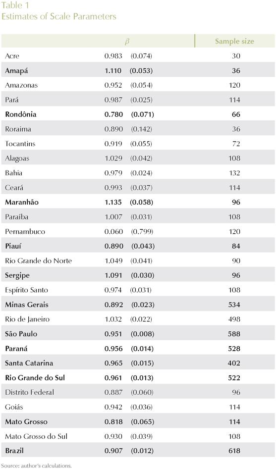
Regressions were estimated considering two different models: fixed effects (FE), and random effects (RE). A Hausman test (HT) for correlation between the error and the regressors was used to check for whether the random effects model was appropriate; the hypothesis that the parameters β and δ are equal to one (constant returns to scale) was tested through the F-test.

The results are presented in Table 1 with the numbers in parentheses indicating standard errors (columns FE and RE), and probability values (columns F-test and HT). Cells, for each state, that are circled, indicate the best method of estimation; shaded cells indicate that the coefficients are statistically different from one (non-constant returns), at 5%.

Results for equation (2), presented in Table 1, reveal evidence of increasing returns in the following states: Minas Gerais, São Paulo, Paraná, Rio Grande do Sul, and Santa Catarina, all located in the more developed Center-South of the country. Also, Rondônia (North), Piauí (Northeast), and Mato Grosso (Center-West) presented evidence of increasing returns. The poor, relatively isolated states of Amapá, Maranhão and Sergipe showed evidence of decreasing returns to scale. Other states did not show evidence of non-constant returns in the manufacturing sector.

B. MODELING OF TRANSPORTATION COSTS

There is not an extensive literature base on which to draw in modeling transportation costs and the impacts of transportation investment in CGE models (for a review, see Kim, Hewings and Hong, 2004; and Kim and Hewings, 2004). The set of equations that specify purchasers' prices in the B-MARIA model imposes zero pure profits in the distribution of commodities to different users. Prices paid for commodity i from region s in region q by each user equate to the sum of its basic value and the costs of the relevant taxes and margin-commodities. This formulation, standard in the preparation in national income and product accounts is not featured in most of the new economic geography models. As McCann (2005) has noted, caution should be exercised in adopting iceberg transportation cost assumptions; he notes that the treatment of geography and space in many of the new economic geography models is very particular and based on assumptions which would be regarded as untenable in most other spatial models. Hence, the preference adopted in this model is for transportation cost specification based on margins.

The role of margin-commodities is to facilitate flows of commodities from points of production or points of entry to either domestic users or ports of exit. Margin-commodities, or, simply, margins, include transportation and trade services, which take account of transfer costs in a broad sense⁵. Margins on commodities used by industry, investors, and households are assumed to be produced at the point of consumption. Margins on exports are assumed to be produced at the point of production. The margin demand equations show that the demands for margins are proportional to the commodity flows with which the margins are associated; moreover, a technical change component is also included in the specification in order to allow for changes in the implicit transportation rate. The general functional form used for the margin demand equations is presented below:

where XMARG(i,s,q,r) is the margin r on the flow of commodity i, produced in region r and consumed in region q; AMARG(i,s,q,r) is a technology variable related to commodity-specific origin-destination flows; η(j,s,q,r) is the margin rate on specific basic flows; X(i,s,q) is the flow of commodity i, produced in region r and consumed in region q; and θ(i,s,q,r) is a parameter reflecting scale economies to (bulk) transportation. In the calibration of the model, θ(i,s,q,r) is set to one, for every flow.

In B-MARIA, transportation services (and trade services) are produced by a regional resource-demanding optimizing transportation (trade) sector. A fully specified PPF has to be introduced for the transportation sector, which produces goods consumed directly by users and consumed to facilitate trade, i.e. transportation services are used to ship commodities from the point of production to the point of consumption. The explicit modeling of such transportation services, and the costs of moving products based on origin-destination pairs, represents a major theoretical advance (Isard et al, 1998), although it makes the model structure rather complicated in practice (Bröcker, 1998b). As will be shown, the model is calibrated by taking into account the specific transportation structure cost of each commodity flow, providing spatial price differentiation, which indirectly addresses the issue related to regional transportation infrastructure efficiency. In this sense, space plays a major role.

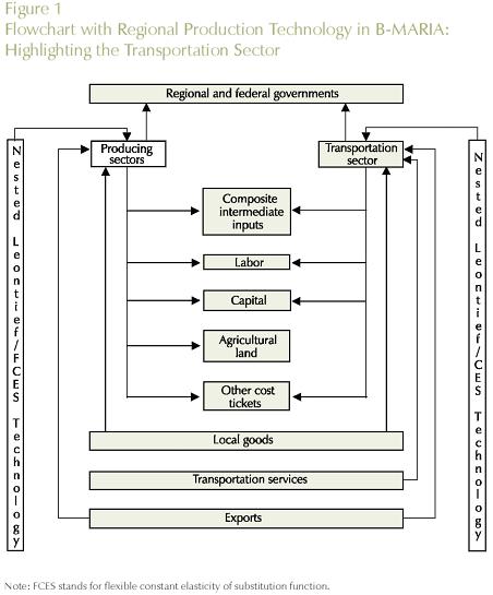
Figure 1 highlights the production technology of a typical regional transport sector in B-MARIA in the broader regional technology. Regional transportation sectors are assumed to operate under constant returns to scale (nested Leontief/CES function), using as inputs composite intermediate goods - a bundle including similar inputs from different sources⁶. Locally supplied labor and capital are the primary factors used in the production process. Finally, the regional sector pays net taxes to Regional and Federal governments. The sectoral production serves both domestic and international markets.

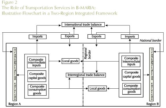
As already mentioned, the supply of the transportation sector meets margin and non-margin demands. In the former case, Figure 2 illustrates the role of transportation services in the process of facilitating commodity flows. In a given consuming region, regionally produced transportation services provide the main mechanism to physically bring products (intermediate inputs, and capital and consumption goods) from different sources (local, other regions, and other countries) to within the regional border. Also, foreign exporters use transportation services to take exports from the production site to the respective port of exit.

The explicit modeling of transportation costs, based on origin-destination flows, which takes into account the spatial structure of the Brazilian economy, creates the capability of integrating the interstate CGE model with a geo-coded transportation network model, enhancing the potential of the framework in understanding the role of infrastructure on regional development. Two options for integration are available, using the linearized version of the model, in which equation (3) becomes⁷:

Considering a fully specified geo-coded transportation network, one can simulate changes in the system, which might affect relative accessibility (e.g. road improvements, investments in new highways). A minimum distance matrix can be calculated ex ante and ex post, and mapped to the inter-regional CGE model. This mapping includes two stages, one associated with the calibration phase, and another with the simulation phase; both of them are discussed below.

1. Integration in the Calibration Phase

In the interstate CGE model, it is assumed that the locus of production and consumption in each state is located in the state capital. Thus, the relevant distances associated with the flows of commodities from points of production to points of consumption are limited to a matrix of distances between state capitals. Moreover, in order to take into account intrastate transfer costs, it is assumed that trade within the state takes place on an abstract route between the capital and a point located at a distance equal to half the implicit radius related to the state area⁸. The transport model calculates the minimum interstate distances, considering the existing road network in 1997.

As Castro, Carris and Rodrigues (1999) observe, road transportation (i.e. truck) is responsible for the largest share of interstate trade in Brazil, accounting for well over 70% of the total value transported. In Brazil's north, however, fluvial transportation is particularly important, but the low quality of the services implies equivalent (high) logistic costs.

The process of calibration of the B-MARIA model requires information on the transport and trade margins related to each commodity flow. Aggregated information for margins on inter-sectoral transactions, capital creation, household consumption, and exports are available at the national level. The problem remains to disaggregate this information considering previous spatial disaggregation of commodity flows in the generation of the interstate input-output accounts. Thus, given the available information - interstate/intrastate commodity flows, transport model, matrix of minimum inter-regional distances and national aggregates for specific margins, the strategy adopted considered the following steps:

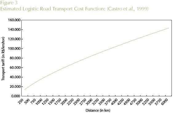
1. In an attempt to capture scale effects in transportation - long-haul economies, a tariff function was used to calculate implicit logistic road transport costs in the interstate Brazilian system⁹. The function considered was estimated by Castro et al. (1999), for 1994, using freight cost data: tariff = 0.25 * dist⁰⁷³, where tariff is the road transportation tariff; and dist refers to the distance between two points. This information was then combined with the matrix of minimum interstate distances to generate a matrix of tariffs evaluated for each path. Long-haul effects are clearly perceived in Figure 3, which plots tariffs for different distances within the relevant range for Brazilian interstate trade.

2. By using such transportation structure, one can capture not only the above-mentioned scale effects, but also relative transfer costs by different origin-destination pairs, which are to be used further on. With that in mind, an index of relative transportation cost was generated. The rows of the tariff matrix were normalized, providing information on differential transportation costs from a given state capital to other state capital, when compared to intrastate costs.

3. The estimates of the various commodity flows at basic values, embedded in the interstate input-output accounts, were then multiplied by the relevant indices from the normalized tariff matrix. This procedure provides the necessary information to generate a distribution matrix, which considers different spatial-destination weights for commodity flows originating in a given state.

4. Finally, the distribution matrix was applied to national totals, considering disaggregated national information on margins by different users, maximizing the use of available information. Further balancing was necessary during the calibration of the model.

In summary, the calibration strategy adopted here takes into account explicitly, for each origin-destination pair, key elements of the Brazilian integrated interstate economic system, namely: a) the type of trade involved (margins vary according to specific commodity flows); b) the transportation network (distance matters); and c) scale effects in transportation, in the form of long-haul economies. Moreover, the possibility of dealing explicitly with increasing returns to transportation is also introduced in the simulation phase, as discussed in the next section. Margin rates are calculated as a mark-up, considering the relation between margins and the respective basic flows.

2. Integration in the Simulation Phase

When running simulations with B-MARIA, one may want to consider changes in the physical transportation network. For instance, one may want to assess the spatial economic effects of an investment in a new highway, expenditures in road improvement, or even the adoption of a toll system, all of which will have direct impacts on transportation costs, either by reducing travel time or by directly increasing out-of-the pocket transfer payments. The challenge becomes one of finding ways to translate such policies into changes in the matrix of minimum inter-regional distances, mimicking potential reductions/increases in the distance between two or more points in space. Such a matrix serves as the basis for integrating the transport model to the inter-regional CGE model in the simulation phase.

One way to integrate both models, in a sequential path, requires the use of either the variable amarg(i,s,q,r) or the parameter θ(i,s,q,r), in equation (3), as linkage variables. Changes in the matrix of inter-regional distances are calculated in the transport model, so that an interface with the inter-regional CGE model is created.¹⁰ As in the specification of the margin demand equations the variable distance is only implicitly portrayed in the parameter η(i, s, q, r), one has to come up with ways in which the information generated by the transport model can be suitably incorporated. Specific transfer rates are present in the model, and changes in them can be easily associated with changes in the matrix of distances.

Let us consider, as an example, a two-region economy, consisted of regions A and B. Let us assume the minimum distance through the existing road network is 100km, on a highway that allows the maximum speed of 50 km/h. Thus, traveling 100 km between A and B takes 2 hours. Moreover, the transfer rate for the only commodity flow, from A to B, is 10%. If the government undertakes a project to improve the A-B link, so that, in the operational phase, maximum speed increases to 80 km/h, a change in the transfer rate due to a change in distance - in our example, travel time reduces to one hour and fifteen minutes (time reduction of 37.5%) - may be estimated, using a model-consistent transfer rate function. A new highway project may also be considered, and a more efficient road design may reduce distance between A and B to, say, 75 km. In this sense, if the new road speed limit is also 50 km/h, one can consider a shortening of distance of 25%. Other similar examples apply.

In the B-MARIA model, information on transfer (trade and transport) rates is available, and so is information on the relevant distances, enabling estimation of a model-consistent transportation cost function. With that in hand, changes in transfer rates can be estimated and incorporated in the interregional CGE model, as follows. Rearranging equation (3), we have:

with θ(i, s, q, r) = 1 implying that the left-hand-side becomes the specific transfer (trade or transport) rate. A percentage change in the transfer rate can then be mapped into the technology variable, AMARG(i,s,q,r). Thus, in percentage-change form, amarg(i,s,q,r) becomes the relevant linkage variable, as:

The parameter θ(i, s, q, r) can also be used in the simulation phase, especially in sensitivity analysis experiments. Suppose, for instance, that scale effects to transportation appear for a given commodity flow, in a specific path. Changing assumptions on the values of θ(i, s, q, r) allows for addressing this issue in a proper way, instead of relying on hypotheses on the linkage variable, AMARG(i,s,q,r). On this issue, Cuk-rowski and Fischer (2000), and Mansori (2003) have shown that these spatial implications are considered in the context of international trade, and therefore, increasing returns to transportation should be carefully considered.

C. THE HOUSEHOLD DEMAND SYSTEM AND WELFARE INDICATORS

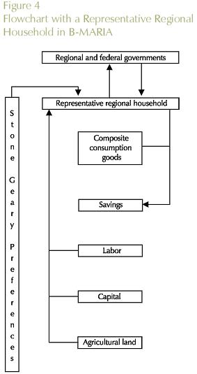
B-MARIA adopts the specification of household demand presented in the MONASH-MRF model (Peter et al, 1996). Consumption is specified via price and expenditure elasticities, which satisfy utility-maximizing conditions. Each representative regional household maximizes a Stone-Geary utility function subject to budget constraint.

Following Horridge (1991), the Stone-Geary or Klein-Rubin per-household utility function, which has the Cobb-Douglas form, is given by:

whereis the aggregate consumption of good i in region r, and(subsistence quantity) and(marginal budget shares on total spending on luxuries) are vectors of parameters. As noted by Peter et al. (1996), a feature of the Stone-Geary utility function is that only the above-subsistence, or luxury, component affects the per-household utility.

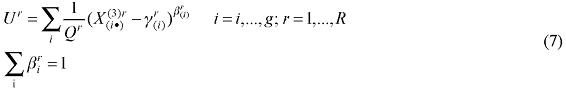
It turns out that the resulting regional demand system implies that the amount spent on each above-subsistence quantity, is a constant share of the total amount spent on above-subsistence goods:

In the B-MARIA model, household preferences are described by a three-level utility function. Together with equation (8), source-specific demand functions, which are specified under the nested structure (Dixon and Rimmer, 2002), determine the composition of household composite good demands. Total household consumption is determined by regional household disposable income, whose definition includes the various components of income and expenditures for the representative households (Figure 4).

1. Measu res of Welfare

The specification of the household demand system in the B-MARIA model allows the computation of measures of welfare. More specifically, one can calculate the equivalent variation (EV) associated with a policy change. The equivalent variation is the amount of money one would need to give to an individual, if an economic change did not happen, to make him as well off as if it did (Layard and Walters, 1978). The Hicksian measure of EV would consider computing the hypothetical change in income in prices of the post-shock equilibrium (Brocker and Schneider, 2002). Alternatively, it can be measured as the monetary change of benchmark income the representative household would need in order to get a post-simulation utility under benchmark prices. More precisely, for homogenous linear utility functions, it can be written as (Almeida, 2003):

where U^r (1) is the post-shock utility; U^r is the benchmark utility; and I^r is the benchmark household disposable income. Note that EV has the same sign as the direction of the change in welfare, i.e. for a welfare gain (loss) it is positive (negative). Aggregate (national) welfare can be assessed by simply summing up the regional EV over r.

Another informative welfare measure refers to the relative equivalent variation (REV). It is defined as the percentage change of benchmark income the representative household would need in order to get a post-simulation utility under benchmark prices (Brocker, 1998). That is:

A. CALIBRATION

Calibration of the household demand system in B-MARIA requires benchmark values for each regional household's income and expenditure flows, which are derived from the SAM database, and estimates for the regional budget shares,(see Dixon, Parmenter, Sutton and Vincent, 1982).

IV. SIMULATIONS

In this section, the main results from the simulations are presented. The basic experiment consisted of the evaluation of an overall 1% reduction in transportation cost within the country. In other words, for every domestic origin-destination pairs, the usage of transportation margins is reduced by 1%. The simulations were carried out under two different economic environments: short-run and long-run. The idea behind this exercise is to assess potential efficiency gains in the transportation network associated with regulation issues, as discussed in the introduction.

A. FUNCTIONING MECHANISME

In this sub-section, we present the main causal relationships underlying the simulation results. The simulation exercise considers an overall reduction in the transportation cost in the Brazilian interstate system. According to the model structure, this represents a margin-saving change, i.e. the use of transportation services per unit of output is reduced, implying a direct reduction in the output of the transportation sector. As shipments become less resource-intensive, labor and capital are freed generating excess supply of primary factors in the economic system. This creates a downward pressure on wages and capital rentals, which are passed on in the form of lower prices. A more comprehensive attempt would need to link this system with a model of the transportation shippers' market to explore the degree to which deregulation would effect downward pressure of transportation costs and the extent to which these changes would or would not been uniform across commodities and interstate routes.

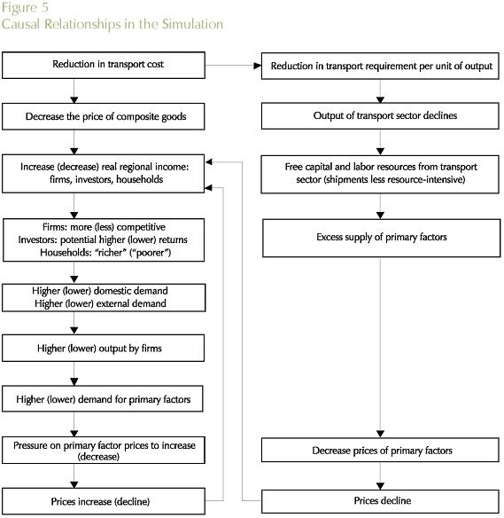
The reduction in transport cost decreases the price of composite commodities, with positive implications for real regional income: in this cost-competitiveness approach, firms become more competitive -as production costs go down (inputs are less costly); investors foresee potential higher returns- as the cost of producing capital also declines; and households increase their real income, envisaging higher consumption possibilities. Higher income generates higher domestic demand, while an increase in the competitiveness of national products stimulates external demand. This creates room for increasing firms' output - directed for both domestic and international markets- which requires more inputs and primary factors. Increasing demand puts pressure on the factor markets for price increases, with a concomitant expectation that the prices of domestic goods would increase.

Second-order prices changes go in both directions - decrease and increase. The net effect is determined by the relative strength of the countervailing forces. Figure 5 summarizes the transmission mechanisms associated with major first-order and second-order effects in the adjustment process underlying the model's aggregate results.

As for the differential spatial effects, three major forces operate in the short-run -two price effects and one income effect- and the net result will heavily depend on the structure of the integrated interstate system. Regarding regional performance, two substitution mechanisms through price effects are relevant to understand the adjustment process. First, there is a direct substitution effect. Consider two trading regions, one exporting and another importing, r and s, respectively. As transportation costs between the two regions go down, r will increase its penetration in s, producing more for s, as it is now cheaper to buy from r. A substitution effect operates in the sense that s will directly substitute output from r for either regional output, or other regions' output (including foreign products).

Moreover, another substitution effect operates. In order to produce for s, r will buy inputs from other regions. As these inputs are now cheaper, due to reductions in transportation costs, region r, with better access to input sources, becomes more competitive, expanding its output. This is the indirect substitution effect.

However, a third countervailing force appears in the form of an income effect. With better accessibility, the demand for products from region r increases. The sources of higher demand for the region's output come from a substitution effect - prices of r's output are now lower - and an income effect - real income increases. This puts pressure on prices, and the net effect will depend on whether the direct and indirect substitution effects will prevail over the income effect.

In the long-run, a fourth mechanism becomes relevant: the "re-location" effect. As factors are free to move between regions, new investment decisions define marginal re-location of activities, in the sense that the spatial distribution of capital stocks and the population changes. The main mechanism affecting regional performance is associated with capital creation. As transportation costs decreases, better access to non-local capital goods increases the rate of returns in the regions. At the same time this potentially benefits capital importing regions, it has a positive impact on the capital-good sectors in the producing regions.

Finally, regions might be adversely affected through re-orientation of trade flows (trade diversion), as relative accessibility changes in the system. Thus, overall gains in efficiency in the transportation sector are not necessarily accompanied by overall gains in welfare. This issue of trade diversion versus trade creation has been an important one in the international trade literature.

B. RESULTS

The presentation of the simulation results is divided into four groups. First, we present the basic results under the long-run closure, focusing on the relevant aggregate variables that help us understanding the functioning mechanism of the model, as described in the previous sub-section¹¹. Spatial effects considering changes in welfare and real GDP are also presented. Secondly, we check the robustness of the results for the key parameters related to the simulation exercises, namely, regional trade elasticities, and parameters to scale economies. To reach this goal, systematic sensitivity analysis is carried out. Thirdly, we take a close look at the long-run results, as they seem to be more closely linked to expected outcomes of transportation policies. Scaffolding of the spatial results is considered in order to evaluate analytically important transportation links to optimize specific policy goals. Finally, as an attempt to better understand the role of increasing returns in the spatial allocation of activities in an integrated inter-regional system, we adjust the parameter of scale economies in the São Paulo manufacturing sector with the idea to check whether, in the Brazilian case, with improvements in transportation, the São Paulo firms have a competitive advantage to further exploit scale economies with reductions in transportation costs, thereby exacerbating the welfare differentials between regions.

1. Basic Results

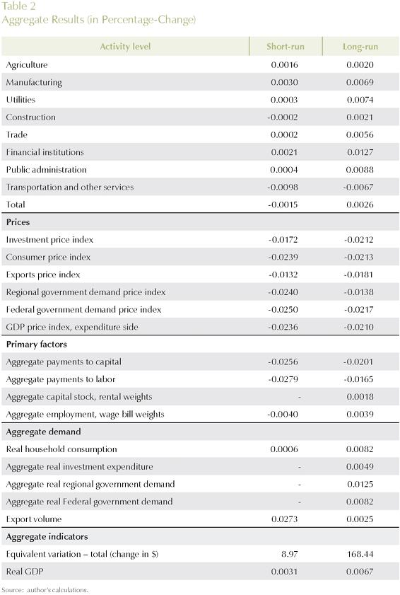
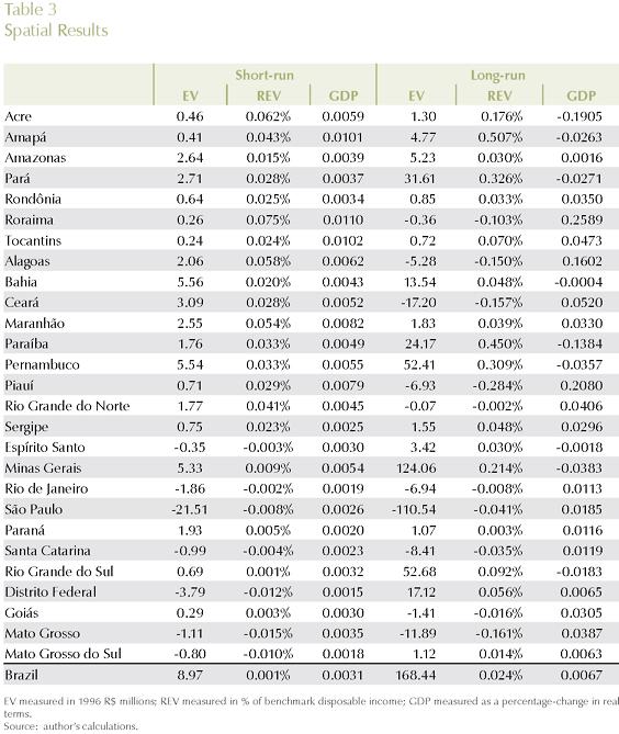
Tables 2 and 3 summarize the results of the two (short-run and long-run) simulations to provide a sense of the outcomes under the different closure rules. These are the only tables in which both sets of results will be presented. Gains in efficiency (real GDP growth) and welfare (equivalent variation) are positive, and magnified in the long-run. Table 3 presents the efficiency and welfare spatial effects. While in terms of efficiency, states in the Center-South seem to have a better performance, in terms of welfare; households in the less developed regions with better access to producing regions appear to be better-off.

2. Systematic Sensitivity Analysis¹²

CGE models have been frequently criticized for resting on weak empirical foundations. While Hansen and Heckman (1996) argue that while the flexibility of the general equilibrium paradigm is a virtue hard to reject, and that it provides a rich apparatus for interpreting and processing data, it can be considered as being empirically irrelevant because it imposes no testable restrictions on market data. McKitrick (1998) has also criticized the parameter selection criteria used in most CGE models, arguing that the calibration approach leads to an over-reliance on non-flexible functional forms.

Although most CGE modelers recognize that accurate parameters values are very important, it is not easy to find empirical estimates of key parameters, such as substitution elasticities, in the literature. Most of the models take up estimates "found in the literature" or even "best guesstimates" (Deardorff and Stern, 1986). Thus, if there is a considerable uncertainty surrounding the "right" parameters, and these are key elements in the CGE results, a consistent procedure in their evaluation is imperative. The problem in CGE models is compounded by the presence of a variety of parameters, some estimated with known probability distributions, others with no known distributions combined with input-output/SAM data that are provided as point estimates (see Haddad et al, 2002).

If a consistent econometric estimation for key parameters in a CGE model study is not possible, the effort should be directed to tests of the uncertainty surrounding these parameters in terms of their impact on the model. Robustness tests are an important step in enhancing the acceptance of the model results in applied economics. The assumptions embodied in CGE models come from general equilibrium theory. However, one set of assumptions, the values of model parameters are natural candidates for sensitivity analysis. Wigle (1991) has discussed alternative approaches for evaluating model sensitivity to parameter values, while DeVuyst and Preckel (1997) have proposed a quadrature-based approach to evaluate robustness of CGE models results, and demonstrated how it could be used for an applied policy model.

The Gaussian Quadrature (GQ) approach (Arndt, 1996; DeVuyst and Preckel, 1997) was proposed to evaluate CGE model results' sensitivity to parameters and exogenous shocks. This approach views key exogenous variables (shocks or parameters) as random variables with associated distributions. Due to the randomness in the exogenous variables, the endogenous results are also random; the GQ approach produces estimates of the mean and standard deviations of the endogenous model results, thus providing an approximation of the true distribution associated with the results. The accuracy of the procedure depends on the model, the aggregation and the simulations employed. Simulations and tests with the Global Trade Analysis Project (GTAP) model, a large-scale model, have shown that the estimates of mean and standard deviations are quite accurate (Arndt and Hertel, 1997).

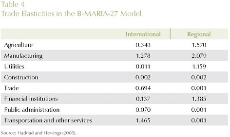
In the B-MARIA-27 model, one set of regional trade elasticities in the Armington demand structure determines the substitution possibilities between goods from different domestic sources. Smaller trade elasticities imply less substitution among regional sources in the model. The change in the results will depend on the interaction of the transportation cost cuts, price responses and these elasticities. Table 4 shows the default values in the aggregation used in this paper. Data from the balanced interstate SAM were extracted to estimate implicit regional trade elasticities, to be used in the calibration of the model. This procedure guarantees data consistency between the SAM database and the estimated parameters. Moreover, it is now possible to provide point and standard error estimates for such key parameters. However, the model-consistent information is not free from the structural constraints imposed during the process of building the SAM; on the other hand, without this information, proper estimation would not be possible. The second group of sensitivity analyses was carried out in the scale economies parameters, µ

The transportation cost reduction experiments discussed above are employed using the Gaussian Quadrature approach to establish confidence intervals for the main results. The range for the elasticities was set to +/- one standard error estimate around the default value, with independent, symmetric, triangular distributions for the two parameters.

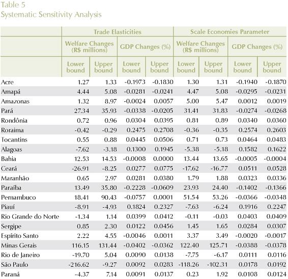
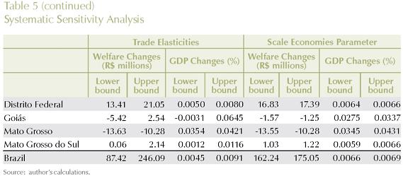
Table 5 summarizes the sensitivity of GDP and welfare results in each Brazilian state for the ranges in the two individual sets of parameters. The lower bound and the upper bound columns represent the 90% confidence intervals for the estimates, constructed using Chebyshev's inequality. We observed that, in general, state results are relatively more robust in the short-run rather than in the long-run and also more robust to scale economies parameters rather than to regional trade elasticities. Overall, the state simulation results can be considered robust to both sets of parameters. In some cases, however, qualitative changes can be observed for the SSA of the trade elasticities: in the long-run, direction of welfare in Rio Grande do Norte, Rio de Janeiro, Paraná, Santa Catarina, and Goiás is inconclusive; direction of GDP growth in the states of Amazonas, Bahia, Pernambuco, Espírito Santo, and Goiás is also inconclusive.

3. Analytically Important Transportation Link

It has been argued that, given the intrinsic uncertainty in the shock magnitudes and parameter values, sensitivity tests are an important next step in the more formal evaluation of the robustness of (inter-regional) CGE analysis and the fight against the "black-box syndrome". However, some important points should be addressed in order to have a better understanding of the sensitivity of the models' results. In similar fashion to the fields of influence approach for input-output models developed by Sonis and Hewings (1992), attention needs to be directed to the most important synergetic interactions in a CGE model. It is important to try to assemble information on the parameters, shocks and database flows, for example, that are the analytically most important in generating the model outcomes, in order to direct efforts to a more detailed investigation¹³.

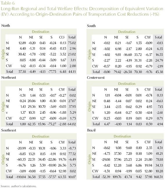
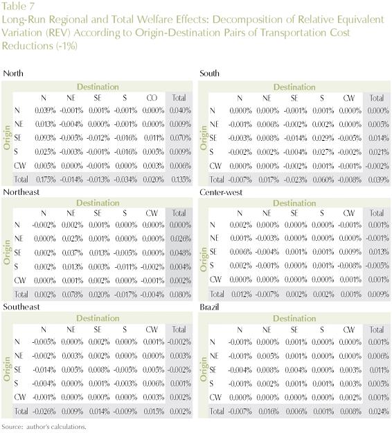
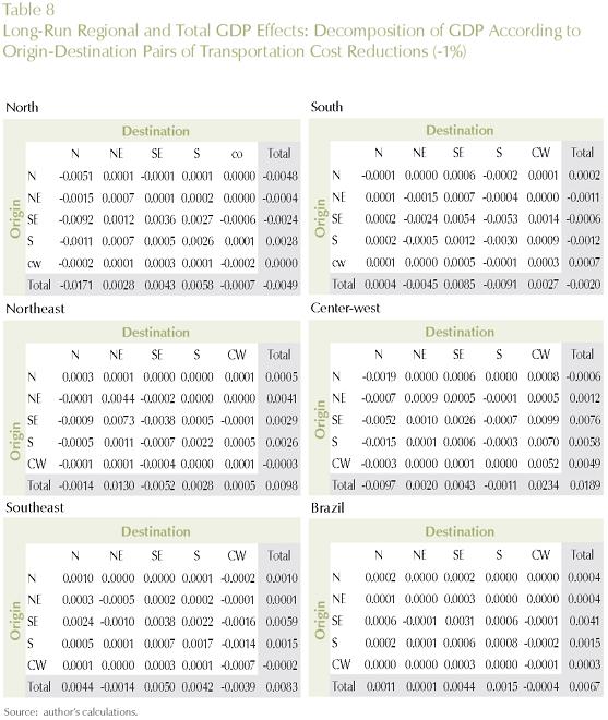
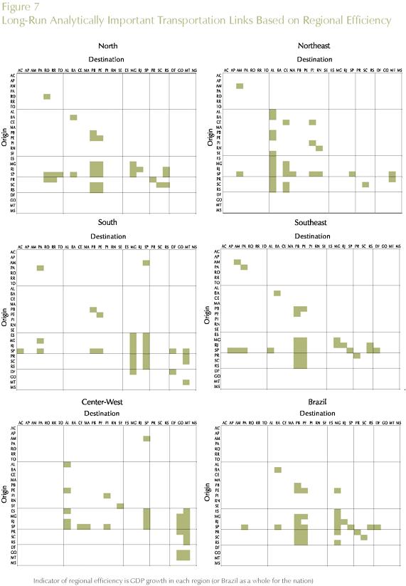
In order to address this issue, in the context of our long-run simulation, we proceeded with a thorough decomposition of the results considering the role played by the various shocks. In other words, we explicitly considered the role played by each transportation link - 27x27 in total - in generating the model's results¹⁴. For each transportation link, we calculated its contribution to the total outcome, considering different dimensions of regional policy. Impacts on regional efficiency and welfare were considered. We looked at the effects on regional efficiency, through the differential impacts on GDP growth for the five Brazilian macro regions (North, Northeast, Southeast, South and Center-West), and for the country as a whole (systemic efficiency). Moreover, we considered the differential impacts on regional welfare, looking at the specific macro regional results, and also at total national welfare.

Tables 6, 7, and 8 present the results for the different policy targets. Transportation links between and within macro regions are explicitly considered, and the estimates of their contributions to the specific policy outcome are presented.

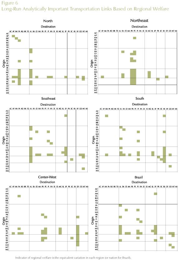
To obtain a finer perspective on the analytically most important transportation links for optimizing a given policy target (regional/national efficiency/welfare), we further decomposed the results into state-to-state links. Key links for each policy strategy (regional/national GDP growth and welfare) are presented in Figures 6 and 7.

4. The Role of Increasing Returns

In inter-regional CGE modeling, another possible way to overcome the scarcity of estimates of regional key parameters is to estimate policy results based on different qualitative sets of values for the behavioral parameters and structural coefficients (Haddad et al., 2002). Through the judgment of the modeler, a range of alternative combinations reflecting differential structural hypotheses for the regional economies can be used to achieve a range of results for a policy simulation. This method, called qualitative or structural sensitivity analysis,¹⁵ provides a "confidence interval" to policy makers, and incorporates an extra component to the model's results, which contributes to increased robustness through the use of possible structural scenarios. As data deficiency has always been a big concern in regional modeling, one that will not be overcome in the near future, this method tries to adjust the model for possible parameter misspecification. If the modeler knows enough about the functioning of the particular national and regional economies, the model achieves a greater degree of accuracy when such procedure is adopted. Qualitative and systematic sensitivity analysis should be used on a regular basis in inter-regional CGE modeling in order to avoid, paradoxically, speculative conclusions over policy outcomes.

Qualitative sensitivity analysis is carried out in this sub-section in order to grasp a better understanding on the role played by the introduction of non-constant returns to scale in the modeling framework. More specifically, the goal here is to assess the role played by increasing returns in the manufacturing sector in the state of São Paulo, the richest, most industrialized state in Brazil and for which there is evidence that it is the focal point of agglomeration economies in the country. For instance, a crude indicator using the PIA data set mentioned above shows that, while São Paulo's share in manufacturing value added in the period 1996-2001 was 47.3%, the state's share in total manufacturing labor was 39.9%.

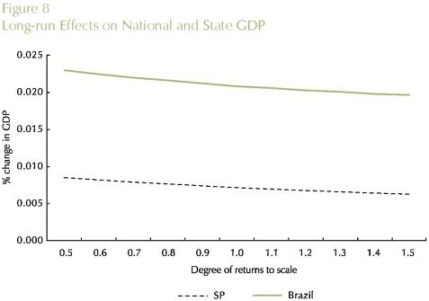
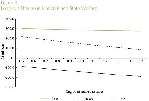
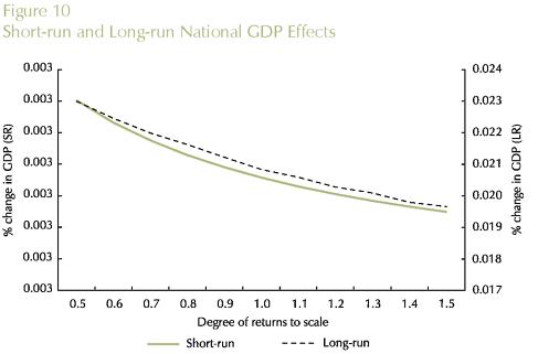
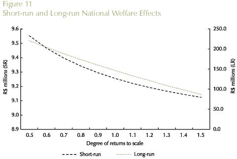
Theoretical results from the new economic geography literature suggest that there is a fundamental trade-off between transportation costs and increasing returns. If this is the case, in a core-periphery inter-regional system, the core region, which hosts the increasing-return sector, can potentially further benefit from improvements in the transportation sector by exploiting scale economies. We check this result using the B-MARIA model with a special set of values for the scale economies parameters; we assume constant returns in every sector in every state. The only exception is the manufacturing sector in the state of São Paulo, for which we consider an interval in the IRTS curve, ranging from high increasing returns (µ = 0.5) to decreasing returns to scale (µ = 1.5), i.e., µ∈ [0.5,1.5 in the manufacturing sector. A series of simulations is run for various vales of µ in the assumed interval. Results are presented in Figures 8 through 11. Theoretical results are confirmed in the empirical experimentation with B-MARIA-27. As it becomes clear from the results for both São Paulo's GDP and welfare, the further down the IRTS curve, the better the state's performance in terms of GDP growth and welfare.

V. FINAL REMARKS

This paper begins an exploration of the Brazilian economy using an inter-regional computable general equilibrium model that is in the process of being unfettered from the reins of the perfectly competitive modeling paradigm. The process is ongoing and difficult; attempts to handle non-constant returns to scale, agglomeration and core-periphery phenomena, imperfect competition, and transportation costs present enormous challenges. Put together, the analysis becomes even more intractable. Further, there is the issue of parameter estimation and sensitivity; some of the analysis in this paper suggests that this area remains contentious.

However, the results provided are encouraging in the sense that the issues, while difficult, are not insurmountable. The challenges to competitive equilibrium in the spatial economy presented by the new economic geography remain largely untested. The present paper offers one approach to a goal of narrowing the gap between theory and empirical application. The Brazilian economy, sharing features of both developed and developing countries, presents a further challenge; the non-uniformity of the spatial distribution of resources and population, the glaring disparities in welfare across states and the presence of a hegemonic economy, in São Paulo, that renders traditional CGE modeling of limited value.

The results reveal that it is possible to handle increasing returns to scale, to address issues of asymmetric impacts of transportation investment and to approach the problems of more flexible functional forms, uncertainties about data and parameter estimates in ways that are tractable and theoretically defensible. The paper offers the perspective that there is a need, perhaps, to pause and take stock of the current state of the art in CGE modeling for multiregional (spatial) economies and to pursue further some of the lines of inquiry initiated by this work.

1 The complete specification of the model is available in haddad and hewings (1997) and haddad (1999).

2 For example, it is typical in long-run comparative-static simulations to assume that the growth in capital and investment are equal (see Peter et al., 1996).

3 The applied models are usually associated with neoclassical assumptions of smooth monotonous convex functions and competitive market assumptions, which allow for a single equilibrium. Instead, one may however use model structures and functional specifications for which existence and uniqueness proofs are not available (Dervis, De Melo and Robinson, 1982). In such cases, finding a solution becomes an empirical question.

4 More precisely, in the standard specification, a nested Leontief/CES function is adopted. It can be shown, though, that the Leontief functional form represents a special case of the CES (see, for instance, Dixon, Bowles and Kendrick, 1983).

5 Hereafter, transportation services and margins will be used interchangeably.

6 The Armington assumption is used here.

7 Equation (12) in the Appendix.

8 Given the state area, we assume the state is a circle and calculate the implicit radius.

9 The general form of transport cost functions (...) is either linear or concave with distance. These reflect the usual empirical observations of the relationship between transport costs and haulage distance (McCann, 2001).

10 This procedure assumes one can translate time distance into Euclidean distance. Ideally, one should use a minimum time distance matrix to avoid shortcomings in the process mentioned above.

11 As noted earlier, the short-run results are the focus in Haddad and Hewings (2005).

12 The discussion below draws on Domingues, Haddad and Hewings (2003).

13 See Domingues et al. (2003).

14 We were able to consider the two-way dimension of a transportation link between to regions, i.e. the way "in" and the way "out".

15 The term "qualitative sensitivity analysis" is used as opposed to "quantitative sensitivity analysis", which is the practice adopted by modelers to define confidence intervals for the simulations' results. Usually, the parameters are allowed to deviate over a range centered in the initial assigned values, or to present small increases/decrease in one direction, which does not address the likely cases of structural misspecifications.

REFERENCES

1. Almeida, E. S. "MINAS-SPACE: A Spatial Applied General Equilibrium Model for Planning and Analysis of Transportation Policies in Minas Gerais", Ph. D. Dissertation, Departamento de Economia/IPE, Universidade de São Paulo, São Paulo (in Portuguese), 2003.         [ Links ]

2. Arndt, C. "An Introduction to Systematic Sensitivity Analysis via Gaussian Quadrature", GTAP Technical Paper No. 2, West Lafayette, Indiana, Center for Global Trade Analysis, Purdue University, 1996.         [ Links ]

3. Bilgic, A.; King, S.; Lusby, A.; Schreiner, D. F. "Estimates of U.S. Regional Commodity Trade Elasticities", Journal of Regional Analysis and Policy, vol. 32, num. 2, 2002.         [ Links ]

4. Brõcker, J. "Operational Computable General Equilibrium Modeling", Annals of Regional Science, num. 32, pp. 367-387, 1998.         [ Links ]

5. Castro, N.; Carris, L.; Rodrigues, B. "Custos de Transporte e a Estrutura Comercial do Comércio Interestadual Brasileiro". Paper presente at the VI Seminário de Acompanhamento do Nê-mesis, December 06-07, IPEA, Rio de Janeiro, 1999.         [ Links ]

6. Cukrowski, J.; Fischer, M. M. "Theory of Comparative Advantage: Do Transportation Costs Matter?" Journal of Regional Science, vol. 40, num. 2, pp. 311-322, 2000.         [ Links ]

7. Deardorff, A. V.; Stern, R. M. The Michigan Model of World Production and Trade. Cambridge, The MIT Press, 1986.Dervis, K. J.; De Melo, J.; Robinson, S.General Equilibrium Models for Development Policy, A World Bank Research Publication, Cambridge, Cambridge University Press, 1982.         [ Links ]

8. DeVuyst, E. A.; Preckel, P. V. "Sensitivity Analysis Revisited: A Quadrature-Based Approach", Journal of Policy Modeling, vol. 19, num. 2, pp. 175-185, 1997.         [ Links ]

9. Dixon, P. B.; Bowles, S.; Kendrick, D. Teoría microeconómica: notas y problemas. Barcelona, Editorial Hispano Europea, 1983.         [ Links ]

10. Dixon, P. B.; Parmenter, B. R.; Powell, A. A.; Wilcoxen, P. J. Notes And Problems In Applied General Equilibrium Economics, Advanced Textbooks in Economics 32, Eds. C. J. Bliss and M. D. Intriligator, North-Holland, Amsterdam, 1992.         [ Links ]

11. Dixon, P. B.; Rimmer, M. T. "Forecasting and Policy Analysis with a Dynamic CGE Model of Australia", G. W. Harrison, S. E. H. Jensen, L. H. Pedersen and T. F. Rutherford, (eds.). Using Dynamic General Equilibrium Models for Policy Analysis, Amsterdam, Elsevier, 2002.         [ Links ]

12. Dixon, P. B.; Parmenter, B. R.; Sutton, J.; Vincent, D. P. ORANI: A Multisectoral Model Of The Australian Economy, North-Holland Amsterdam, 1982.         [ Links ]

13. Domingues, E. P. "Regional and Sectoral Dimensions of FTAA", Ph. D. Dissertation, Departamento de Economia/IPE, Universidade de São Paulo, São Paulo (in Portuguese), 2002.         [ Links ]

14. Domingues, E. P.; Haddad, E. A.; Hewings, G. J. D. "Sensitivity Analysis in Applied General Equilibrium Models: An Empirical Assessment for MERCOSUR Free Trade Areas Agreements", Discussion Paper 04-T-4, Regional Economics Applications Laboratory, University of Illinois, Urbana., 2003.         [ Links ]

15. Fujita, M.; Krugman, P.; Venables, A. J. The Spatial Economy: Cities, Regions and International Trade, Cambridge, MIT Press, 1999.         [ Links ]

16. Fujita, M.; Thisse, J-F. Economics of Agglomeration, Cambridge, University Press, 2002.         [ Links ]

17. Haddad, E. A. Regional Inequality and Structural Changes: Lessons from the Brazilian Experience, Aldershot, Ashgate, 1999.         [ Links ]

18. Haddad E.A.; Azzoni, C. R. "Trade Liberalization and Location: Geographical Shifts in the Brazilian Economic Structure", J.J.M. Guilhoto and G.J.D. Hewings (eds), Structure and Structural Change in the Brazilian Economy, Alders-hot, Ashgate, 2001.         [ Links ]

19. Haddad, E. A.; Domingues, E. P. "EFES - Um Modelo Aplicado de Equilíbrio Geral para a Economia Brasileira: Projeções Setoriais para 1999-2004", Estudos Econômicos, vol. 31, num. 1, 2001.         [ Links ]

20. Haddad, E. A.; Hewings, G. J. D. "Market Imperfections in a Spatial Economy: Some Experimental Results", The Quarterly Review of Economics and Finance, num. 45, pp. 476-496, 2005.         [ Links ]

21. Haddad, E. A.; Hewings, G. J. D.; Peter, M. "Input-Output Systems in Regional and Interregional CGE Modeling", G. J. D. Hewings, M. Sonis and D. Boyce (eds.), Trade, Networks and Hierarchies, Berlin, Springer-Verlag, 2002.         [ Links ]

22. Hansen, L. P.; Heckman, J. J. "The Empirical Foundations of Calibration". The Journal of Economic Perspectives, vol. 10, num. 1, pp. 87-104, 1996.         [ Links ]

23. Harrison, W. J.; Pearson, K. R.; Powell, A. A. "Multiregional And Inter-temporal AGE Modelling Via GEMPACK", Preliminary Working Paper no. IP-66, IMPACT Project, Monash University, Clayton, September, 1994.         [ Links ]

24. Hertel, T. W. E.; Tsigas, M. "Structure of GTAP", T. W. Hertel (ed.), Global Trade Analysis: Modeling and Applications, Cambridge University Press, 1997.         [ Links ]

25. Isard, W. Location and the Space Economy, Cambridge, MIT Press, 1959.         [ Links ]

26. Isard, W.; Azis, I. J.; Drennan, M. P.; Miller, R. E.; Saltzman, S.; Thorbecke, E. Methods of Interregional and Regional Analysis, Ashgate, 1998.         [ Links ]

27. Kim, E.; Hewings, G. J. D.; Hong, C. "An Application of Integrated Transport Network -Multiregional CGE Model I: A Framework for Economic Analysis of Highway Project", Economic Systems Research, num. 16, pp. 235-258, 2004.         [ Links ]

28. Kim, E.; Hewings, G.J. D. "An Application of Integrated Transport Network -Multiregional CGE Model II: Calibration of Network Effects of Highway", Discussion Paper, 04-T-xx, Regional Economics Applications Laboratory, University of Illinois, Urbana. www.uiuc.edu/unit/real, 2004        [ Links ]

29. Mansori, K. F. "The Geographic Effects of Trade Liberalization with Increasing Returns in Transportation", Journal of Regional Science, vol. 43, num. 2, pp. 249-268, 2003.         [ Links ]

30. McCann, P. Urban and Regional Economics. Oxford University Press, 2001.         [ Links ]

31. McCann, P. "Transport Costs and the New Economic Geography", Journal of Economic Geography, num. 5, pp. 305-318, 2005.         [ Links ]

32. McKitrick, R. R. "The Econometric Critique of Computable General Equilibrium Modeling: The Role of Functional Forms", Economic Modelling, vol. 15, num. 4, pp. 543-573, 1998.         [ Links ]

33. Peter, M. W.; Horridge, M.; Meagher, G. A.; Na-qvi, F.; Parmenter, B. R. "The Theoretical Structure Of MONASH-MRF", Preliminary Working Paper no. OP-85, IMPACT Project, Monash University, Clayton, April, 1996.         [ Links ]

34. Schmutzler, A. "The New Economic Geography", Journal of Economic Surveys, vol. 13, num. 4, pp. 357-379, 1999.         [ Links ]

35. Whalley, J.; Trela, I. Regional Aspects of Confederation, vol. 68 for the Royal Commission on the Economic Union and Development Prospects for Canada. University of Toronto Press, Toronto, 1986.         [ Links ]

36. Wigle, R. "The Pagan-Shannon Approximation: Unconditional Systematic Sensitivity in Minutes", Empirical Economics, num. 16, pp. 35-49, 1991.         [ Links ]

APPENDIX A

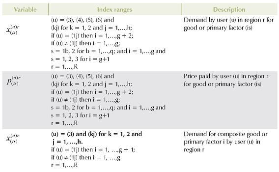
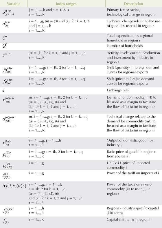
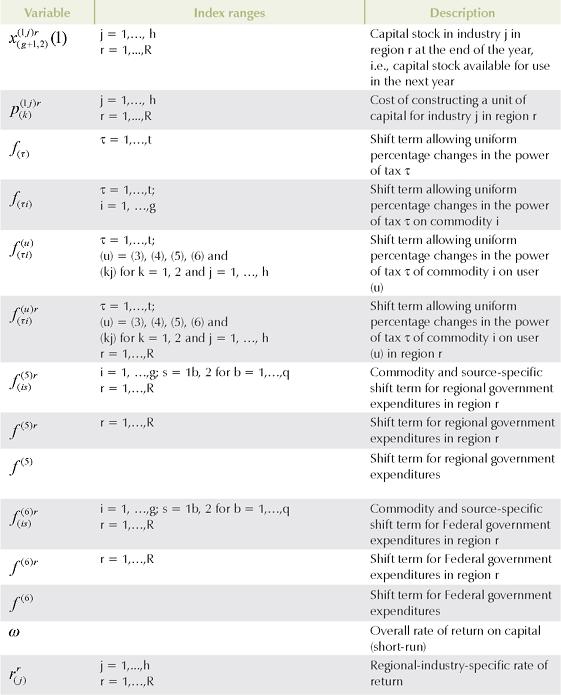
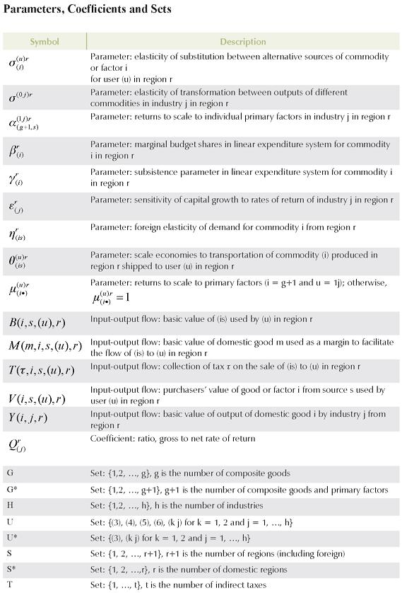
The functional forms of the main groups of equations of the interstate CGE core are presented in this Appendix together with the definition of the main groups of variables, parameters and coefficients.

The notational convention uses uppercase letters to represent the levels of the variables and lowercase for their percentage-change representation. Superscripts (u), u = 0, 1j, 2j, 3, 4, 5, 6, refer, respectively, to output (0) and to the six different regional-specific users of the products identified in the model: producers in sector j investors in sector j (2j), households (3), purchasers of exports (4), regional governments (5) and the Federal government (6); the second superscript identifies the domestic region where the user is located. Inputs are identified by two subscripts: the first takes the values 1, g, for commodities, g + 1, for primary factors, and g + 2, for "other costs" (basically, taxes and subsidies on production); the second subscript identifies the source of the input, being it from domestic region b (1b) or imported (2), or coming from labor (1), capital (2) or land (3). The symbol (•) is employed to indicate a sum over an index.

Equations

Substitution between products from different regional domestic sources

i = 1,..., g; b = 1,q; (u) = 3 and (kj) for k = 1 and 2 and j = 1,h; r = 1,R Substitution between domestic and imported products

i = 1,..., g; s = 1 • and 2; (u) = 3 and (kj) for k = 1 e 2 and j = 1,..., h; r = 1,R Substitution between labor, capital and land

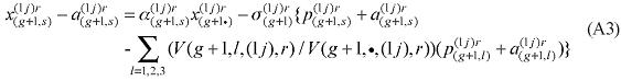
j=1,... , h; s=1, 2 and 3; r=1,... , R

Intermediate and investment demands for composite commodities and primary factors

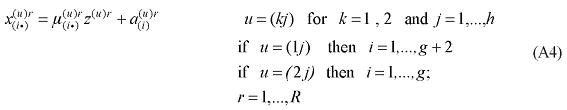
Household demands for composite commodities

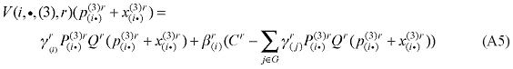
i = 1,...,g ; r = 1,R Composition of output by industries

j = 1,..., h; i = l,...,g; r = 1,R Indirect tax rates

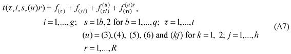
Purchasers' prices related to basic prices, margins (transportation costs) and taxes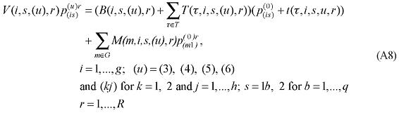

Foreign demands (exports) for domestic goods

Regional government demands

Regional government demands

Margins demands for domestic goods

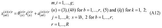
Demand equals supply for regional domestic commodities

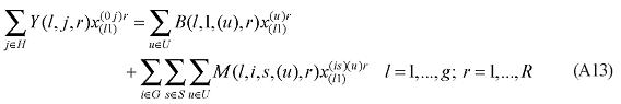
Regional industry revenue equals industry costs

Basic price of imported commodities

Cost of constructing units of capital for regional industries

j = 1,..., h; r = 1,R

Investment behavior

Capital stock in period T+1 - comparative statics

Definition of rates of return to capital

Relation between capital growth and rates of return

Other definitions in the CGE core include: revenue from indirect taxes, import volume of commodities, components of regional/national GDP, regional/national price indices, wage settings, definitions of factor prices, and employment aggregates.

Variables