Martha R. López Juan David Prada^*

^* We would like to thank Andrés Gonzalez, Hernando Vargas, George McCandless, and Hernán Rincón for their comments on earlier drafts. The remaining errors are ours. The views expressed in the paper are those of the authors and do not represent those of the Banco de la República or its Board of Directors. The authors are respectively, Professional Expert and Professional Department of Macroeconomic Models, Banco de la República (Central Bank of Colombia).

E-mail: mlopezpi@banrep.gov.co jpradasa@banrep.gov.co

Document received: 02 June 2009; final version accepted: 07 December 2009.

The unfolding of the 2007 world financial and economic crisis has highlighted the vulnerability of real economic activity to strong fluctuations in asset prices. Which is the optimal monetary policy in an economy like the Colombian that is exposed to swings in asset prices? What is the implication, in terms of central bank losses, when it follows a standard simple rule instead of the optimal monetary policy? To answer these questions, we use a Dynamic Stochastic General Equilibrium (DSGE) model with physical capital and sticky wages for the Colombian economy and derive the optimal monetary policy. Then, we explore the dynamic effects of news about a future technology improvement, which turns out ex post to be overoptimistic, under the optimal policy rule and under alternative specifications of simple rules and definitions of the output gap.

JEL classification: E44, E52, E61.

El desarrollo de la crisis financiera y económica mundial que inició en el 2007 puso en evidencia la vulnerabilidad de la actividad económica real ante fluctuaciones marcadas en los precios de los activos. ¿Cuál es la política monetaria óptima en una economía como la colombiana, expuesta a cambios significativos en los precios de los activos?¿Cuáles son las implicaciones, en términos de pérdidas del Banco Central, cuando se sigue una regla simple y estándar en lugar de la política monetaria óptima? Para darle respuesta a estas preguntas utilizamos un modelo dinámico y estocástico de equilibro general (DSGE, por sus siglas en inglés) con capital físico y salarios rígidos para la economía colombiana, buscando obtener como resultado la política monetaria óptima. A continuación, analizamos los efectos dinámicos de una noticia sobre una futura mejora tecnológica —que posteriormente resultó demasiado optimista— bajo la regla de la política óptima y, de manera alternativa, bajo especificaciones de reglas simples y definiciones de la brecha de producción.

Clasificación JEL: E44, E52, E61.

O desenvolvimento da crise financeira e econômica mundial que iniciou em 2007 pôs em evidência a vulnerabilidade da atividade econômica real frente a flutuações marcadas nos preços dos ativos. Qual é a política monetária ótima em uma economia como a colombiana, exposta a mudanças significativas nos preços de dos ativos? Quais são as implicações, em termos de perdas do Banco Central, quando se segue uma regra simples e padrão em vez da política monetária ótima? Para dar resposta a estas perguntas utilizamos um modelo dinâmico e estocástico de equilíbrio geral (dsge, pelas suas siglas em inglês) com capital físico e salários rígidos para a economia colombiana, buscando obter como resultado a política monetária ótima. A continuação analisamos os efeitos dinâmicos de uma notícia sobre uma futura melhora tecnológica —que posteriormente resultou demasiado otimista— sob a regra da política ótima e, de maneira alternativa, sob especificações de regras simples e definições da brecha de produção.

Classificação JEL: E44, E52, E61.

During the last couple of decades, many monetary authorities around the world have achieved the goal of a low and stable inflation rate. However, this price stability has not come hand in hand with higher asset price stability. Borio and Filardo (2003), among others, document the emergence of asset prices and credit and investment booms and busts, which have become a more important source of macroeconomic instability in both developed and developing countries. Financial unbalances are of great concern because when they unwind, the real economy is exposed to a substantial economic downturn and, very frequently, to recession; for example, many economists attribute at least some part of the 1990 recession in the United States to the preceding decline in commercial real estate prices (Bernanke and Gertler 1999).

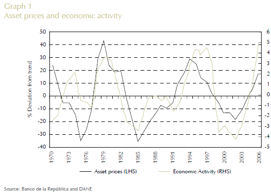
Colombian economy, as many other developing economies, has experienced very strong asset prices and output fluctuations. Graph 1 displays the cyclical component of economic activity and asset prices for the Colombian economy during 1970-2005¹ . Two boom and bust episodes are evident; the first during the eighties and the second during the nineties. A boom phase occurred in 2004, followed by an economic downturn triggered by the 2007 global financial crisis. The close correlation between asset prices cycles and the output cycle, and the evidence of a financial accelerator mechanism in the Colombian economy found by López, Prada and Rodriguez (2008), raises the question if the nature of monetary policy can explain the behavior of both variables. Would the boom and bust cycles be smoother if the monetary authority incorporated a response to asset prices in the simple monetary policy rule? How costly, in terms of the central bank loss function, is a monetary policy that reacts only to inflation and output gaps instead of taking into account asset prices?

To answer these questions, we set up a model for the Colombian economy where, as in Cristiano, Ilut, Motto and Rostagno (2008), the boom phase is triggered by a signal that leads agents to rationally expect an improvement in technology in the future, but which turns out to be false, and the bust phase of the cycle begins when people find this out. We explore the effects of this news about a future technology improvement, which turns out ex post to be overoptimistic, under the optimal policy rule and under alternative specifications of simple rules.

By optimal monetary policy we mean a policy that minimizes an intertemporal loss function under commitment. The intertemporal loss function is a discounted sum of expected future period losses. We choose two alternative welfare criteria. The first is a quadratic period loss function that corresponds to flexible inflation targeting and is the weighted sum of two terms: the squared inflation gap between inflation and the inflation target, and the squared output gap between output and potential output. The second measure of loss that we consider is a utility-based loss function.

As in Svensson et al. (2008), a key issue for a flexible inflation targeting central bank is which measure of output gap should try to stabilize. We report results from three alternative concepts of gap used in the loss functions and in the simple policy rules. The first concept is the deviations of output and asset prices from the hypothetical level that would exist if the economy would have had flexible prices and wages. The second is the deviations from steady-state values. The third concept (used only in the simple rules) corresponds to growth rates.

The model we use is a DSGE model for a small open economy as the one in Colombia. The model distinguishes households and entrepreneurs. Households consume and work, while entrepreneurs produce a homogeneous intermediate good using capital bought from capital producers and labor supplied by households. Entrepreneurs take bank loans, facing borrowing constraints tied to the value of collateral. In addition, there are banks, who offer two types of financial assets to agents: saving and loans; retailers, who set the final price of output goods; workers, who supply their differentiated labor services through a union that sets wages to maximize its members´ utility, generating a nominal rigidity in wages, à la Calvo. There is also a foreign sector which provides assets at the foreign interest rate which is positively related to the domestic´s economy net foreing asset position. Finally, there are capital producers, who transform output goods into capital goods; a government, and a central, bank which conducts monetary policy.

The remainder of the paper is as follows; Section II describes the model. Section III presents the optimal policy problem, the different simple rules and the alternative results of a boom and bust episode. Section IV concludes.

A. HOUSEHOLDS AND WAGE SETTING

1. Consumption and saving decisions

The domestic economy is inhabited by a continuum of households indexed by i ε [0, 1].. The representative agent i maximizes the following utility function:

where c^pc_t (i) is per capita consumption, h^pc_t (i) is per capita hours worked, and l^pc_t (i) is per capita leisure time, which satisfies l^pc_t (i) = t − h^pc _t (i),, with t > 0 being the total endowment of time. N_t is the total population, which follows a stochastic process.

The discounted utility is given by:

with σ > 0. ς > 0 and φ > 0. Parameter ς is the inverse elasticity of labor supply with respect to real wages. Parameter σ is the constant relative risk aversion coefficient. Preferences display habit formation in consumption governed by parameter φ. χ^u,h_t are the preferences shocks that shift the consumption demand and leisure, and A_t represents productivity, which follows the process:

where ε^A_t is a white noise variable.

Following Prada (2008), we assume that there exist transaction costs in the economy. The exchange process requires real resources. In this process, the more transactions involved, the higher the transaction cost, and the higher the deposits held by households, the lower the transaction cost:

where v_t (i) is deposits velocity and d^h_t−1 (i) are the deposits held by household i.

Cost per unit of transaction is given by ϑ (v_t (i)),, an increasing, positive, twice differentiable, convex function. In particular, we assume that:

Households´ decisions have to match the following budget constraint:

where (a_t (i)) represents Arrow-Debreu assets with price p^a_t (i), (d^h _t (i)) the deposits, (τ_t) the lump-sum taxes, (w_t) the real wage, ( tr_t) the foreign transfers, (II_t) the total profits from firms and banks ownership, ( i^d _t−1) the interest on bank deposits and (π^{c t} ) the CPI inflation rate.

Households choose consumption and the composition of their portfolios by maximizing (1) subject to (4). Given that we are assuming the existence of Arrow-Debreu assets, consumption is equalized across households and the first order conditions can be expressed in terms of effective worker:

along with (4), where λ_t is the budget constraint Lagrange multiplier.

2. Labor supply and wage setting

Following Erceg et al. (2000), we assume that a continuum of monopolistically competitive households supply differentiated labor services to the production sector as an imperfect substitute for the labor services of other households. There is a set of perfect competitive labor service assemblers that combines household´s labor hours in the same proportions as firms would choose. The aggregator´s demand for each household´s labor demand is defined as:

The optimal composition of this labor service unit is obtained by minimizing its cost, given the different wages set by different households. The demand for each differentiated variety of labor is given by:

where is an aggregate wage index and θ^w > 0 is the elasticity of substitution among labor varieties.

We assume that wage setting is subject to a nominal rigidity, à la Calvo (1983). The duration of each wage contract is randomly determined: in any given period, the household is allowed to reset its wage contract; also, with probability (1− ε^w), the household is not allowed to reset its wage contract. We assume there is an updating rule for all those households that cannot reoptimize their wages. In particular, if a household cannot reoptimize during i periods between t and t + i, then its wage at t + i, is given by:

where n ∈ N is the indexation horizon, γk ≥ 0 is the weight assigned to inflation rate k periods earlier and 1 − ∑ⁿ_m=1 γ_wm ≥- 0 is the weight assigned to the target inflation set by the monetary authority, π.. This adjustment rule implies that workers who do not optimally reset their wages update them by using a geometric weighted average of past CPI inflation and the inflation target set by the Central Bank, π.

Any period of time t , in which a household is able to reset its wage contract, solves the problem:

subject to the labor demand (8), the updating rule for the nominal wage (9) and the budget constraint (4).

B. EBTREPRENEURS

Entrepreneurs purchase capital in each period, and use it in combination with hired labor, h_t to produce the intermediate product, q^s_t, following a constant returns to scale technology:

where The intermediate product is sold in a competitive market at wholesale price, p^qs_t. Following Christiano et al. (2008), we assume that technology, χ^qs_t ,, follows the exogenous process given by:

where ε_t and ε_t are uncorrelated over time and with each other. This simple process allows incorporating a boom and bust episode in the model. Throughout the analysis, we consider the following impulse; Up until period 1, the economy is in steady state. In period t = 1, there is a signal that suggests ln ( χ^qs_t ) will be high in period 1 + p. But, when period 1 + p occurs, the expected rise in technology in fact does not happen.

Capital stock depreciates at the rate δ > 0. Following Gerali et al. (2008), we assume that in order to finance capital purchases entrepreneurs have access to loan contracts offered by banks. The amount of resources that banks are willing to lend to entrepreneurs, z^f_t, is constrained by the value of their collateral, which is given by their holdings of physical capital. The borrowing constraint is:

where m^f_t is the loan-to-value ratio and i^zf_t is the interest rate paid on loans. The entrepreneur´s budget constraint is:

where II^qs_t represents the flow of profits that will be transferred to households.

Given labor demand, the representative firm purchases k^s_t+1 units of capital, at price p^k_t, to maximize its expected sum of profit flows, using as the appropriate discount factor. Optimality conditions are given by:

Retailers buy output from entrepreneurs and slightly differentiate it at no resource cost. The differentiation of output gives the retailers some market power. Households and firms then purchase CES aggregates of these retail domestic goods. Retailers are introduced to motivate sticky prices and we follow Calvo (1983) in introducing price inertia. Each retailer faces a demand for variety j given by:

Following Calvo (1983), we assume that only a fraction (1− ε^q) of sellers is allowed to reset their prices. In particular, if a firm cannot set an optimal price, then it follows a nonoptimal price rule:

where n ∈ N is the indexation horizon, γk 0 is the weight assigned to the inflation rate k periods earlier and 1 − ∑ⁿ_m=1 γ_qm ≥ 0 is the weight assigned to the target inflation set by the monetary authority, π.

If the firm receives a signal to optimally adjust its price, it will choose p^q_t (j) to maximize:

D. CAPITAL PRODUCERS

Capital producers purchase consumption goods as a material input, x_t, and combine it with the existing capital stock, to produce new capital. We assume that capital producers are subject to quadratic capital adjustment costs. The price of capital is determined by a q-theory of investment.

The aggregate capital stock evolves according to:

where χ^k_t is the marginal efficiency of investment, following Greenwood et al. (1988). Capital producers´ optimization problem, in real terms, consists of choosing the quantity of investment to maximize profits, so that:

subject to (18). The K_t-1 - first order condition is:

E. BANKS

The banking industry is assumed to be perfectly competitive. Since economic agents require deposits and credit, banks produce the financial services through a production technology that uses real resources from the economy as an input. Following Edwards and Vegh (1997), the production technology for banks is given by the cost function:

ξ_tη(z^f_t, d_t)

which is positive for z^f_t, d_t > 0, convex, continuously differentiable, increasing in all arguments, and homogeneous of degree one.

ξ_t represents an inverse measure of the total productivity of the banking intermediation sector. It is a cost scale factor exclusive of the banking sector that follows that process:

-ln (ξ_t) = (1 − ρ_ξ) ln ξ - + ρ_ξ ln (ξ_t−1) + ε^ξ_t

where ξ is the expected value of the cost scale factor, ρ_ξ ∈ [0, 1) and ε^ξ is a white noise variable with variance σ²_ξ .

The policy of the Central Bank and the banking sector is related through the reserve requirement, which is a fixed proportion τ^d_t > 0 of total deposits, so the bank reserves, rbt,, satisfy the constraint:

rb_t ≥ τ^d_t d_t (21)

Banks can borrow from the Central Bank at a nominal rate, i^bc_t. The net debt of a private bank with the Central Bank is bt.. Banks also finance themselves through foreign debt, ft, and they pay the interest rate, i^f_t , set in the foreign market. It is assumed that the banks are the only private agents that have access to foreign resources.

The representative bank seeks the maximization of the discounted sum of profits (II^b_t). . The bank´s resource constraint is given by:

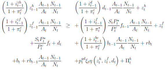
The bank´s income is given by credit interest payments at a nominal rate i^zf_t−1, foreign debt accumulation f_t, deposits accumulation dt,, accumulation of debt with the Central Bank b_t and the returned reserve from the Central Bank rb_t−1. These revenues are used to pay for deposits at an interest rate i^d_t, to accumulate credit z^f_t , to pay foreign debt at the interest rate i^f_t−1, to pay the interest to the central bank i^cb_t, to accumulate new reserves, to pay the real cost of the financial intermediation and to make profit transfers to households, ^b_t. 1 +π^*_t represents the foreign inflation rate.

The production technology of the financial services is represented by the cost function:

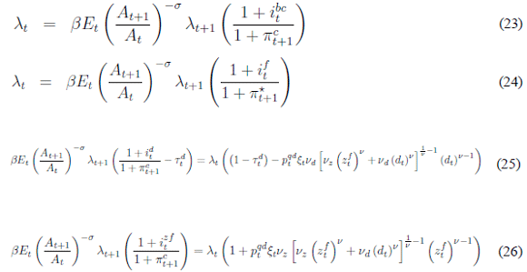
The bank´s optimization problem is a dynamic process. Banks maximize expected value of the discounted sum of profit flows. The relevant discount factor is The first order conditions for domestic, foreign debt accumulation, deposits, and credit are:

F. FOREIGN SECTOR

Following Schmitt-Grohé and Uribe (2003), we assume that the foreign sector provides resources to the economy at the interest rate, i^f_t , that depends on total net foreign indebtedness, f − a_t^bc, as a percentage of GDP, y_t, as follows:

Where i^* is the risk-free foreign interest rate, χ^if_t is a foreign interest rate shock, a_t^cb are foreign assets held by the Central Bank, is the steady state value of net foreign assets and Ω _u > 0 is a scale parameter. We close the model in this way because without it, net foreign indebtedness might be nonstationary, complicating the analysis of local dynamics. In steady state, and 1 +i^f = (1 + i^*) χ^if .

G. CENTRAL BANK

Monetary authority is able to set the nominal interest rate prevailing in the interbank market, i^bc_t , following a Taylor-type rule:

where ρ_π and ρ_y are, respectively, the weights assigned to inflation and output stabilization, εⁱ_t is an exogenous shock to monetary policy and y^flex_t represents the hypothetical output level that would exist if the economy would have had flexible prices and wages.

The resource constraint of the Central Bank is given by:

where a^bc_t is the exogenous stock of foreign net assets and II^bc_t are the transfers to the government.

H. GOVERNMENT

The government obtains resources from lump-sum taxes, τ_t, and net transfers from the Central Bank, the transaction costs, and capital adjustment, and uses this to finance public expenses, g_t which follow the process:

where is the expected value of the government expenditure, ρ_g∈ (0, 1) and ε^g are white noise with variance σ²_g.

I. NATIONAL ACCOUNTS

Real GDP, y_t, the final domestic income of the households:

from which we can define trade balance as:

Where tr_t represents foreign transfers.

J. MODEL PARAMETRIZATION

The model is calibrated to match key steady-state ratios of Colombia. In the model, a period corresponds to one quarter.

1. Long-run parameters

Following Mahadeva and Parra (2008), the annualized foreign steady-state real interest rate faced by the Colombian economy is set at 3.42%. This implies a discount factor of β =0.999. Following Prada (2008), the value of n is set to match the average annual rate of growth of the total population in Colombia, 1.22%, and the parameter a is calibrated to obtain an annual rate of growth of the labor-augmenting productivity of 1.5%. A value of σ = 2 is used as the constant relative risk aversion coefficient, Arias (2000).

The steady-state foreign annual inflation rate is set at 2% and the domestic annual rate is set at 3%, the long-run target of the Central Bank in Colombia. The parameter ς is set at 3 to obtain a Frisch elasticity of 0.33, close to the value found by Prada and Rojas (2009).

The model is calibrated to produce a steady state-value of h =0.294, the share of time dedicated to the labor market. This implies a value of χ^h =146.90. We assume that banking costs are quadratic, and set ν = 2. To match the average annualized real lending rate (7.92%) and the average annualized real deposit rate (2.01%) reported in Prada (2008), we set ν_d = 6.284 × 10−5 6.284 x 10^-5 and ν_z = 1.324 × 10⁻⁴.

In the level of real GDP, the steady state is normalized to unity. This is achieved by setting χ^qs = 0.524.. The exogenous public expenditure parameter, g, is calibrated to obtain a steady-state ratio of government expenditure to GDP of , equal to the average of that ratio in the period 1994:1-2007:4.

Following Mahadeva and Parra (2008), the value of total foreign net assets to GDP is set to 1.20, and this implies a value of 1.20 for the parameter . The average ratio of net foreign assets of the Central Bank to GDP (net foreign assets, monetary sectorization - Banco de la República) is 0.454 in the period 2005:1 - 2007:4, and the parameter a^cb is set to match this ratio.

The average ratio of net foreign transfers to GDP is 0.0351 and the parameter tr is set to this value. We assume quadratic transaction costs and set ϑ₁ = 2.. The parameter ϑ₀ is calibrated to match the value of the average ratio of deposits that generate costs to the banks to GDP (1.20). This implies a value of ϑ₀ = 0.0126. The parameter α = 0.456 is calibrated to get the average ratio of investment to GDP (0.215), reported in Prada (2008). The steady-state leverage ratio m^f is calibrated to match the average ratio of credit to GDP (2.10). This implies m^f = 0.33.. Following Prada (2008), τ^d is set at 0.062 and a^cb is set at 0.454.

2. Short run and additional parameters

Following Arango et al. (1998) the markup on the marginal cost of production is set at 25%, and this implies a value of θ^q = 5. The same markup is assumed for the wage setting process. Following Bonaldi et al. (2009), the Calvo parameters that measure the degree of price stickiness are selected in such a way that, on average, the final price of the good is adjusted once each year (ε^q =0.75) and the wage rate is adjusted once each four months (ε^w =0.25). The elasticity of substitution between labor and capital is set at ρ =0.84, as in Bonaldi et al. (2009).

In the baseline calibration it is assumed that there is no monopolistic competition in the financial system, because this condition is not needed to explain the spread between interest rates. Then, θ^d —› ∞ - and θ^z —› ∞. The habit persistence φ is set at 0.5. The parameter of the adjustment cost of investment Ψ^X is set at 0.7. The persistence of the exogenous processes is 0.6. The parameters of the policy rule are standard: ρi =0.75, ρ_π =1.25 and ρ_y= 10.50.

We find the Ramsey optimal allocations for our economy using the computer code and the strategy used in Levin and Lopez-Salido (2004), and Levin et al. (2005). The Central Bank minimizes an intertemporal loss function at time t:

where

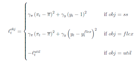
where flex represents the flexible price equilibrium variables and ss stands for steady-state values. The first two losses are often used as a metric for capturing policymaker´s preferences in studies that attempt to evaluate the trade-off between inflation variability and output variability. In addition to these losses, we consider a second measure of loss: i.e., a utility-based loss function, which we denote −ℓ^util_t. Following [Woodford (2001)], we derive ℓ^util_t by taking a second order log-linearization of the utility function around the steady state. We ignore the constant and first order terms (the latter are zero in unconditional expectation) and focus on the unconditional expectation of the second order terms. The result is:

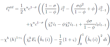
The terms that appear in the utility-based loss function, are directly related to the distortions present in our model; the welfare of the representative consumer is adversely affected by variability in consumption and the dispersion of hours worked between households (similarly to Levin et al. 2005).

The minimization of the loss function is subject to the DSGE model described before. The optimization results in a set of first order conditions, which combined with the model equations yields a system of difference equations that can be solved using several alternative algorithms.

On the other hand, we close the model with alternative simple rules and compare the results when a bubble shock occurs. The first policy rule that we examine is the flexible price rule eq. (28), where the Central Bank responds only to inflation and output gaps (defined as deviations from the flexible price equilibrium). In the second policy rule used in the simulations the monetary policy also reacts directly to asset prices:

The third and fourth rules are similar to the simple the rule, eq. (28) and eq. (30), but instead of using deviations of output and asset prices from the flexible price equilibrium, we use the output growth rate and the asset prices growth rate, as follows:

Finally, we use two simple rules where the output and the asset price gaps are defined as deviations from steady-state values (ss).

A. RESULTS FOR BOOM AND BUST

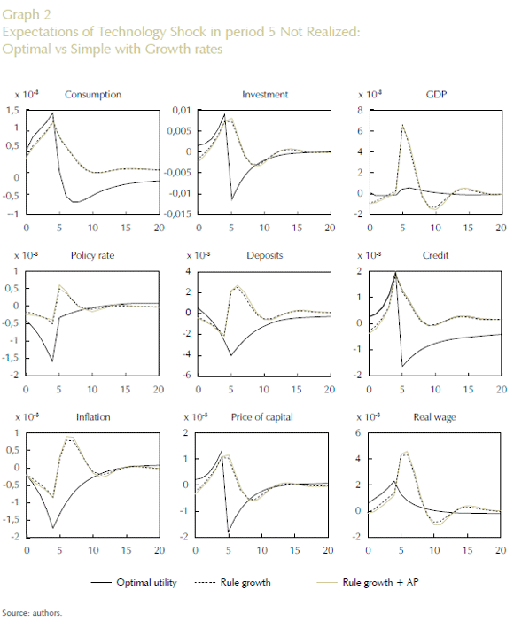
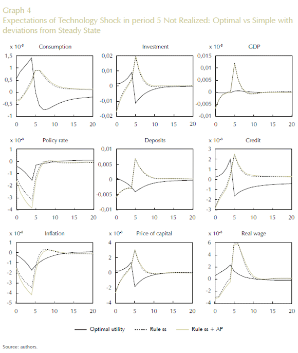
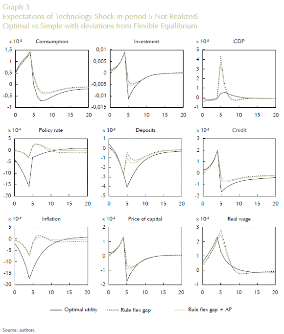
The results in Graphs 2-4 show the dynamic response of our model to a ε_t shock that occurs in period 1, followed by e_t = −ε_t+p for p = 5.. Thus, there is a signal that technology will improve in the future that turns out to be false in the end. A positive signal arriving in t − p indicates households that the economy is likely to be more productive p periods ahead. Anticipating this, they try to bring the future value of more production to the present. They increase consumption and investment, in preparation for the future expected increase in productivity. To finance these activities, households increase their demand for credit and assets. Capital price rises due to the expected need for new capital in the future. This constitutes the boom stage of the cycle, based solely on expectations. But p periods ahead, when productivity is supposed to change, a surprise shock, ε_t , may occur. For instance, if ε_t = −e_t−p, then productivity stays still and the expected productivity change does not happen. This might happen, for instance, if a new technology results less efficient than expected, or if a production policy fails after generating good signals. Then, households face the consequences of higher consumption and investment financed through credit, without real support. The economy enters a recession: consumption, investment, asset prices and general economic activity fall. The boom has been burst.

We compare the dynamic properties of output, consumption, investment, asset prices, nominal interest rate, real wages, deposits, credit and inflation in the Ramsey equilibrium with the behavior of these variables when we close the model with alternative simple policy rules. Graph 2 shows the dynamic response of these variables for the Ramsey equilibrium and for the model closed with the simple rule that reacts to the output and inflation growth rates and with the rule that also reacts to the asset price growth rate, with ρ_pk =0.5. With a monetary authority that follows a simple rule, a minor fluctuation is transformed into a substantial boom and bust cycle. This happens, firstly, because the real wage rises during the boom in the Ramsey equilibrium, and so, an efficient way to achieve a higher real wage is to let inflation drop; but the monetary authority, who follows the inflation targeting strategy, is reluctant to let this happen, and instead, responds to inflation weakness by shifting to a looser monetary policy stance. Secondly, when the productivity shock does not occur, the Central Bank does not react fast enough in relation to the optimal policy, causing a higher volatility.

Letting a reaction from Central Bank to asset price gap does not significantly improve the dynamics of the variables, but as we will see later, when we compare the rules in terms of central bank losses there exist an important difference.

Graph 3 plots the results of the policy rule that takes into account output and asset prices deviations from the flexible economy. The boom and bust is smoother in this case because the boom is shorter than in the case of the flexible price rules shown in Graph 2. The worse scenario occurs in the case where the monetary authority uses an instrument rule that reacts to deviations of output and asset prices from steadystate values, Graph 4. In this case, the dynamic of the series is much more volatile. In addition, when the productivity shock turns out to be false, the monetary authority reacts too slowly in relation to the flexible price rule. In terms of these responses this is the less desirable type of rule. The most suited policy rule, which is closer to the optimal policy, is the simple rule that reacts to the output gap and the asset price gap using deviations from the flexible-price economy.

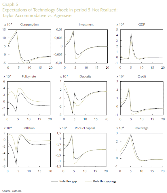
Something worth noting is that if the monetary policy is more aggressive (ρ_π =2.25) than accommodative (ρ_π =1.25) -in terms of targeting inflation- in the rule that uses deviations from the flexible equilibrium economy, the volatility of output and inflation is reduced, as can be seen in Graph 5. Therefore, we compute the losses for the different types of rules for both cases, the accommodative and the aggressive monetary policy.

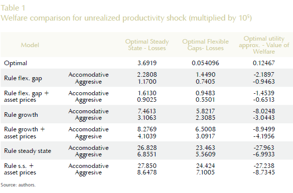
Table 1 below shows the results for the three alternative criteria of welfare for the alternative simple rules under accommodative and aggressive policy rules. The optimal policy using deviations from flexible prices in the loss function is the one that delivers the lower losses.

As can be seen, the lower losses are obtained with the flexible price rules with an aggressive monetary policy. Rules that perform the worst are those where the monetary authority responds to deviations of output and asset prices from steady-state values.

When the Central Bank follows a policy rule, an aggressive stance against inflation seems to better control better the effects of the bubble, in terms of central bank losses. This happens because an aggressive stance allows a lower variability of inflation. A tighter control of prices does not allow the bubble to build up, so the relevant gap of asset prices is lower in the aggressive case. This, in turn, reflects in a slower growth of investment and output when the bubble is building up, and generates a deeper fall of the relevant gap of these aggregates when the bubble bursts.

If the Central Bank does not follow an optimal policy for the three objective functions, the best results are achieved when the bank follows a rule that takes into account deviations of output and asset prices with respect to their hypothetical paths in an economy with flexible prices. Since the expectational shock is real by nature, the economy with flexible prices has similar effects: an increase in gross production, consumption, investment, and domestic and foreign debt. The Central Bank that takes into account that the flexible-price real variables are deviated as well will try harder to control prices and to make real variables behave as in the flexible-price economy. Therefore, it allows a lower variability of prices and a faster fall of consumption, investment and credit when the productivity shock does not occur. This fast adjustment is reflected in less variability of real GDP and generates a smaller loss.

We must note that the dynamics of the economy do not change by much if the central bank takes into account or not the asset prices in the policy rule. The only case in which targeting the price of assets decreases the loss of the Central Bank for the unrealized productivity shock is when the policy rule looks at the flexible-price economy. In this case, the relative improvement from including asset prices is of 32 percent when the loss function uses flexible equilibrium variables. For all the remaining rules, targeting the asset prices does not decrease the loss. Just as before, if the Central Bank targets deviations of asset prices, it will not allow for a fast adjustment. In the case of the flexible-price economy the asset prices fall sharply, and the rule that follows this information will do a fast adjustment.

In conclusion, a fast adjustment of the economy is needed to minimize the loss of the Central Bank when it is obvious that the productivity shock did not really happen.

We calibrated a DSGE model for the Colombian economy that incorporates features such as sticky prices and wages, a banking sector and a financial fragility describing balance sheet effects. We use the model to compute the optimal policy response of the economy under an expectation shock of improvement in technology, which turns out to be false. The benchmark Ramsey-optimal equilibrium is used to compare simple policy rules that monetary authorities might use in the implementation of monetary policy. We find out that the simple policy rule that reacts to deviations of output from potential output —defined as the hypothetical output level that would exist if the economy would have had flexible prices— is the one that delivers the lowest central bank losses. This is because a fast adjustment of the economy is needed when it is obvious that the productivity shock did not happen. Adding asset price gaps to the policy rule does not improve much the dynamics of the economy, unless the Central Bank is able to identify asset price misalignments. Finally, an aggressive monetary policy -in terms of fighting inflation rate- reduces central bank losses, given that output and inflation variability is reduced.

¹ Asset prices correspond to a weighted average of equity prices and real state prices.

1. Arias, A. F. "The Colombian Banking Crisis: Macroeconomic Consequences and What to Expect", Borradores de Economía, no. 157, Bogotá, Banco de la República, 2000.         [ Links ]

2. Bernanke, B.; Gertler, M. "Monetary Policy and Asset Price Volatility", Economic Review, v. 84, no. 4, Federal Reserve Bank of Kansas City, pp. 17-52, 1999.         [ Links ]

3. Arango, J. P.; Gracia, O. ; Hernández, G.; Ramírez, J. M. "Reformas comerciales, márgenes de beneficio y productividad en la industria colombiana", Archivos de Economía, no. 82, Bogotá, Departamento Nacional de Planeación, 1998.         [ Links ]

4. Bonaldi, P.; González, A.; Prada, J.D.; Rodríguez, D.; Rojas, L. "Método numérico para la calibración de un modelo DSGE", Borradores de Economía, no. 548, Bogotá, Banco de la República, 2009.         [ Links ]

5. Borio, C.; William, E.; Filardo, A. "A Tale of Two Perspectives: Old or New Challenges for Monetary Policy?", Working Paper, no. 126, Bank of International Settlements, 2003.         [ Links ]

6. Calvo, G. A. "Staggered Prices in a Utility Maximizing Framework", Journal of Monetary Economics, vol. 12, no. 3, Elsevier, pp. 383-398, 1983        [ Links ]

7. Dixit, A. K.; Stiglitz, J. "Monopolistic Competition and Optimum Product Diversity", American Economic Review, vol. 67, no. 3, American Economic Association, pp. 297-308, 1977.         [ Links ]

8. Christiano; Ilut, L. C.; Motto, R.; Rostagno, M. "Monetary Policy and Stock Market Boom-Bust Cycles", Working Paper, no. 955, European Central Bank, 2008.         [ Links ]

9. Erceg, C.; Henderson, D.; Levin, A. "Optimal Monetary Policy with Staggered Wage and Price Contracts", Journal of Monetary Economics, vol. 46, no. 2, Elsevier, pp. 281-313, 2000.         [ Links ]

10. Edwards, S.; Vegh, C. "Banks and Macroeconomic Disturbances under Predetermined Exchange Rates", Journal of Monetary Economics, vol. 40, no. 2, Elsevier, pp. 239-278, 1997.         [ Links ]

11. Gerali, A.; Lippi, F. "Optimal Control and Filtering in Linear Forward-Looking Economics: A Toolkit", Discussion Paper (mimeo), Banca d´Italia, 2002.         [ Links ]

12. Gerali, A.; Neri, S.; Sessa, L.; Signoretti, F. "Credit and Banking in a DSGE Model" (mimeo), Banca d´Italia, 2008.         [ Links ]

13. Greenwood, J.; Hercowitz, Z.; Huffman, G. "Investment, Capacity Utilization, and the Real Business Cycle", American Economic Review, vol. 78, no. 3, American Economic Association, pp. 402-4178, 1988.         [ Links ]

14. Levin, A. T.; López-Salido, D. "Optimal Monetary Policy with Endogenous Capital Accumulation" (manuscript), 2004.         [ Links ]

15. Levin, A.; Onatski, A.; Williams, J.; Williams, N. "Monetary Policy under Uncertainty in Micro- Founded Macroeconometric Models", Working Paper, no. W11523, National Bureau of Economic Research, 2005.         [ Links ]

16. López, M.; Prada, J. D.; Rodríguez, N. "Financial Accelerator Mechanism in a Small Open Economy", Borradores de Economía, no. 525, Bogotá, Banco de la República, 2008.         [ Links ]

17. Mahadeva, L.; Parra, J. C. "Testing a DSGE Model and its Partner Database", Borradores de Economía, no. 479, Bogotá, Banco de la República, 2008.         [ Links ]

18. Prada, J. D. "Financial Intermediation and Monetary Policy in a Small Open Economy", Borradores de Economía, no. 531, Bogotá, Banco de la República, 2008.         [ Links ]

19. Prada, J. D.; Rojas, L. E. "La elasticidad de Frisch y la transmisión de la política monetaria en Colombia", Borradores de Economía, no. 555, Bogotá, Banco de la República, 2009.         [ Links ]

20. Schmitt-Grohé, S.; Uribe, M. "Closing Small Open Economy Models", Journal of International Economics, vol. 61, no. 1, Elsevier, pp. 163-185, 2003.         [ Links ]

21. Söderlind, P. "Solution and Estimation of RE Macromodels with Optimal Policy", European Economic Review, vol. 43, nos. 4-6, Elsevier, pp. 813-823, 1999.         [ Links ]

22. Svensson, L. "Optimization under Commitment and Discretion, the Recursive Saddlepoint Method, and Targeting Rules and Instrument Rules: Lecture Notes", 2007.         [ Links ]

23. Svensson, L.; Malin, A.; Laséen, S.; Lindé, J. "Optimal Monetary Policy in an Operational Medium- Sized DSGE Model" (manuscript), 2008.         [ Links ]

24. Woodford, M. "Inflation Stabilization and Welfare", Working Paper, no. W8071, National Bureau of Economic Research, 2001.         [ Links ]