Luis Fernando Gamboa, Andrés García-Suaza, Jesús Otero*

* Faculty of Economics, Universidad del Rosario, Bogotá, Colombia. We would like to thank Russell Davidson, Luis Eduardo Fajardo, Ana María Iregui (Editor), Jeremy Smith and an anonymous referee for their useful comments and suggestions. The usual disclaimer applies. E-mails: luis.gamboa@urosario.edu.co; andres.garcia66@urosario.edu.co; jesus.otero@urosario.edu.co (corresponding author)

Document received: 23 february 2010; final version accepted: 18 may 2010.

This paper uses Colombian household survey data collected over the 1984-2005 period to estimate Gini coefficients and their corresponding standard errors. We find a statistically significant increase in wage income inequality following the adoption of the liberalization measures during the early 1990s, and mixed evidence from the recovery years that followed the economic recession during the late 1990s. We also find that in several cases the observed differences in the Gini coefficients across cities have not been statistically significant.

JEL classification: C12; D31; I32

Este artículo usa información recolectada a través del Sistema de Encuestas de Hogares en Colombia para el periodo 1984-2005 con el fin de estimar coeficientes de Gini y sus errores estándar correspondientes. Encontramos un aumento estadísticamente significativo en la medida de desigualdad salarial, consecuencia de las medidas de liberalización económica adoptadas al comienzo de los años noventa, así como evidencia mixta durante los años de recuperación que siguieron a la recesión económica de finales de esta misma década. Además, encontramos que en muchos casos las variaciones observadas entre los coeficientes de Gini de las diferentes ciudades y a través del tiempo no son significativas en términos estadísticos.

Clasificación JEL: C12; D31; I32.

Este artigo estima coeficientes de Gini para a Colômbia, com seus correspondentes erros padrão, utilizando informação proveniente das Pesquisas de Opinião de Lares durante o período 1984-2005. Encontra-se um incremento estatísticamente significativo na desigualdade do salário por hora no período posterior à abertura econômica do começo da década dos noventa; para os anos posteriores à recessão de finais dos anos noventa, a evidência não é concluinte. Também se encontra que as diferenças observadas nos indicadores de desigualdade entre cidades não foram estatísticamente significativa em vários casos.

Classificação JEL: C12; D31; I32.

Measuring the evolution of income distribution over time and/or across regions and assessing the effect of policy measures on income concentration are topics of research that have historically received a great deal of attention. To address these topics, authors typically provide comparisons based on the ranking of estimated Gini coefficients without acknowledging the fact that, being a sample statistic, these coefficients have associated sampling distributions; see e.g., Baer and Maloney (1997), Caselli and Battini (2000), and Ezcurra and Pascual (2009).

A number of authors have considered different methodologies to estimate the standard error of the Gini coefficient: Zheng and Cushing (2001), Giles (2004 and 2006), Ogwang (2000, 2004 and 2006), and Modarres and Gastwirth (2006). However, in a recent paper Davidson (2009) points out that the estimators available in the literature are either mathematically complex to calculate or quite unreliable. For example, Davidson (2009) shows that the jackknife estimator of the variance is not a consistent estimator of the asymptotic variance of the Gini coefficient, and therefore does not give reliable inference. Davidson (2009) presents a procedure to compute an asymptotically correct standard error for the Gini coefficient based on a relatively simple expression. The work by Davidson has at least three main contributions. First, it provides a bias-corrected estimator of the Gini coefficient. Second, it derives an approximation for the standard error of the Gini coefficient that expresses it as a sum of independent and identically distributed (iid) random variables. Third, it illustrates how bootstrap methods can be used to yield reliable inference about the Gini coefficient.

This paper uses Colombian household survey data collected over the 1984-2005 period to estimate the Gini coefficient for labor income in the urban labor market, as well as for the labor markets in the main seven urban areas. Rankings of Gini coefficients based on income distributions for Colombia have been undertaken by Berry and Urrutia (1976) and Birchenall (2001, 2007), among others. In sharp contrast to this literature, in this paper we estimate standard errors on Gini coefficients. This enables us to test for statistical variation across urban areas and over time. The chosen sample period is interesting because the Colombian government instituted a series of major liberalizing reforms during the early 1990s, although this was followed by the deepest recession experienced by the country in the last century and the subsequent years of recovery.

The paper is organized as follows: Section II briefly describes the methodology used for the estimation of the Gini coefficient and its corresponding standard error. Section III describes the data set and summarizes the main results. Section IV concludes.

The Gini coefficient, defined as twice the area between the equidistribution line (i.e., the 45o line) and the Lorenz (1905) curve, is perhaps the most commonly used measure of inequality. It ranges between zero (perfect equality) and one (perfect inequality). Recently, Davidson (2009) expressed the Gini coefficient as:

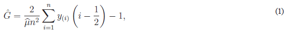
where, y_(i), i = 1,2,.., n, is the series of order statistics of the income variable y (that is, the original series sorted in increasing order), and is the estimated mean of y. Davidson (2009) finds an approximate expression for the bias of G, from which he derives the following bias-corrected estimator of the Gini coefficient, denoted G which is given by:

While the estimator (2) is still biased, its bias is of order smaller than n^-1 Equation (2) can be used to obtain an estimate of the standard error of G Using:

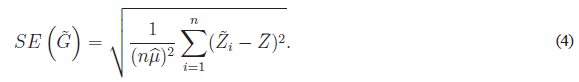
Davidson (2009) shows, via simulation experiments, that the asymptotic distribution of the Gini coefficient is reliable even for sample sizes of around 100 observations. However, in case the underlying income distribution follows a lognormal distribution with a large variance or when the distribution has heavy tails, reliable inference can be obtained by applying the bootstrap method. In particular, Davidson (2009) suggests implementing the bootstrap method as follows. First, let

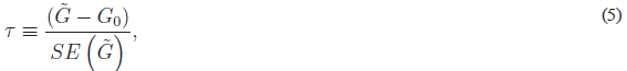
be the test statistic required to test the null hypothesis that the bias-corrected Gini coefficient is equal to G_o Then, one generates b= 1,..., B bootstrap samples of size n by resampling with replacement from the observed income data (which is also of size n ). For bootstrap sample b, one computes a bootstrap statistic T^*_b as in (5), but with G_o replaced by G, that is the value of the statistic computed from the observed sample. This is required so that the hypothesis tested should be true of the bootstrap data-generating process. To calculate an interval at nominal confidence level (1 − α) one estimates the α/2 and 1 − α/2 quantiles of the empirical distribution of the bootstrap statistics T^*_b.

We use data from the nationwide household surveys periodically undertaken by the Departamento Administrativo Nacional de Estadística (DANE). Our period of analysis, i.e., 1984 to 2005, is characterized by the implementation of two different surveys, namely the Encuesta Nacional de Hogares (ENH) and the Encuesta Continua de Hogares (ECH). The former was applied quarterly from 1979 to 2000, and up until 1983 it included the four main cities of Colombia: Bogotá, Medellín, Cali, and Barranquilla. In 1984 three more cities were added to the ENH: Bucaramanga, Manizales, and Pasto. In 2001, the ENH was superseded by the ECH, which is a monthly survey of thirteen cities: the original seven plus Ibagué, Montería, Cartagena, Pereira, Villavicencio, and Cúcuta¹.

The dataset used in the analysis consists of the hourly wage per worker (in constant prices of 2005) during the 1984-2005 period, which is used as a proxy for labor income. The choice of this variable has three important implications for the analysis. First, hourly wage per worker exhibits less variation than personal income. Indeed, over the period from 1984 to 2005 the coefficient of variation of the former ranges from 1.1 to 2.4, while the corresponding coefficient of variation of the latter ranges from 1.2 to 3.2. This implies that Gini coefficients based on hourly wage per worker will be lower than those based on personal income. Second, calculations not reported here suggest that problems of censored and truncated data are more frequent when dealing with personal income than with our measure of hourly wage per worker. For example, in 2001 and 2002 the percentage of individuals who do not report income amounts to approximately 43% and 44%, respectively, while the corresponding percentages for the individuals who do not report wage are 19% and 21%, respectively. Third, the use of hourly wage per worker offers the advantage that it controls for the fact that an individual may earn several wages from different jobs.

The unit of analysis is the employed individuals. This means that individuals who report having worked during the previous week but do not report labor income are excluded from the sample. One might be inclined to think that individuals in the upper tail of the income distribution do not tend to report their income. However, results not reported here indicate that there is no statistical difference between individuals who report labor income and those who do not report it, once one controls for human capital variables, such as education and experience. Furthermore, given that in this paper we are interested in assessing changes in Gini coefficients over time and across cities, it is likely that underreporting will be randomly distributed within the sample.

The data for each year in the 1984-2005 period were obtained by aggregating the surveys of every given year. We use the seven main cities that are available throughout the sample period: Bogotá, Medellín, Cali, Barranquilla, Bucaramanga, Manizales, and Pasto. These account for more than seventy percent of the country's total urban population.

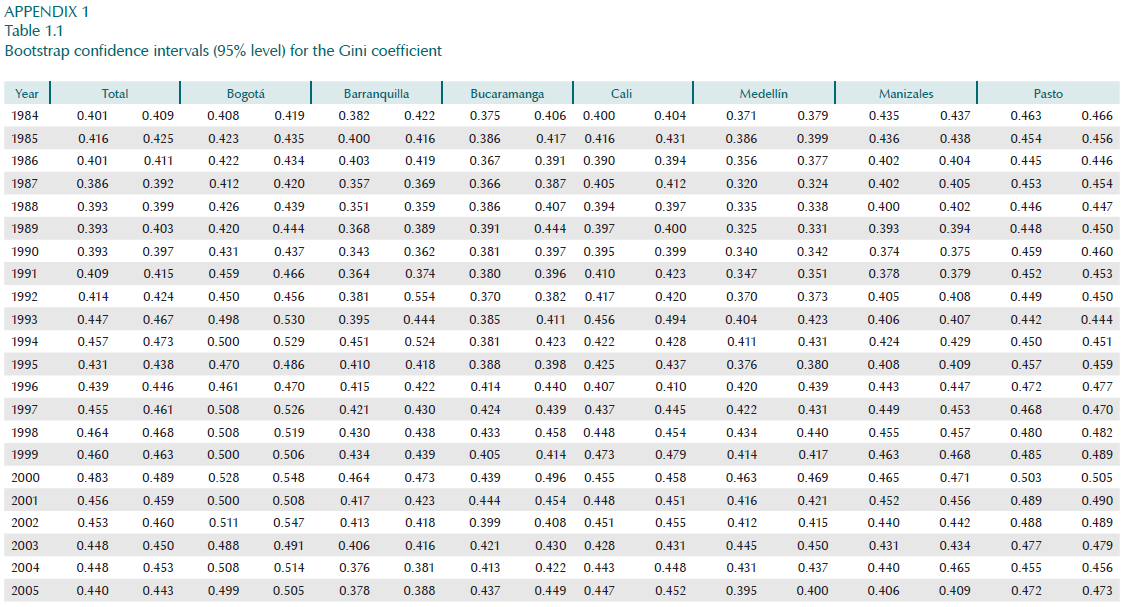
Table 1 reports bias-corrected Gini coefficients for the main seven cities and for the country².

This table also contains the corresponding standard errors based on equation (4), which can be used to construct confidence intervals using the quantiles of the standard normal distribution. The standard errors that result from implementing the bootstrap procedure outlined in the previous section (using 9.999 bootstrap replications) are reported in the Appendix. At this point it is also worth mentioning that the application of the jackknife method results is much larger estimates of the variance of the bias-corrected Gini coefficients; indeed, when using the data for all seven cities the estimated jackknife variance is almost 1.8 times the estimated asymptotic variance derived by the formula given in Davidson (2009)³.

Table 2 reports the number of times the bias-corrected Gini coefficients between pairs of cities are statistically the same over the sample period under consideration, 1984-2005. For example, when looking at Bucaramanga and Barranquilla, in 11 out of the 21 possible cases the coefficients between these two cities do not appear to be statistically different. This table shows that there are only three pairs of cities, namely Bogotá-Medellín, Medellín-Pasto and Bucaramanga-Pasto, for which the estimated coefficients always appear to be statistically different throughout the sample period.

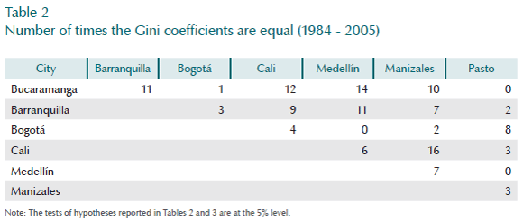
Table 3 compares the evolution of the Gini coefficients for each city and for the country, with respect to three different base years: 1984, 1990 and 1999. The first base year is chosen simply because it is the beginning of our sample period. The second base year allows us to compare with respect to the year when the government introduced a series of structural policy measures aimed at liberalizing Colombian trade and foreign exchange transactions, which were also accompanied by legislation to free the labor market while granting greater protection to union rights (see Urrutia (1994) for a review of these policy reforms). The third base year allows us to provide a comparison with respect to the lowest point of the most serious recession recorded during the last century.

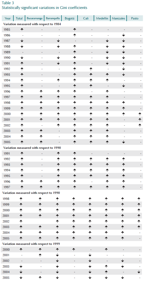
Let us consider first the results when using 1984 as base year. The cities of Barranquilla, Medellín and Manizales exhibit a downward trend in their Gini coefficients during the 1980s and early 1990s, which is subsequently reversed starting in the mid- 1990s. In the case of Pasto, wage income distributions appear not to have changed with respect to the level observed in 1984. In the cases of Bogota and the aggregate of the seven cities, the corresponding Gini coefficients appear to have moved upwards.

Using 1990 as base year, we find that most of the Gini coefficients exhibit an increase. This suggests that the liberalizing policy reforms of the early 1990s led to a worsening distribution of income. Lastly, when looking at the period that followed the deepest recession of the last century, evidence is somewhat mixed. The years of recovery do not appear to have had an effect on wage income distribution in 21 out of the 48 comparisons provided, whereas in 18 cases there is a statistically significant fall in the Gini coefficients.

Overall, when assessing variations in the distributions of wage income with respect to 1990 and 1999, the picture that emerges is not particularly optimistic in the sense that most of the observed variations in the Gini coefficients are in the positive direction (reflecting a worsening in inequality). It appears that the best-case scenario is that which reflects no statistically significant variation at all.

This paper analyses the evolution of the Gini coefficient in Colombia across cities, as measured by the hourly wage per worker, over a period of more than two decades. To provide valid inference on the observed variations of the estimated Gini coefficients, we implement the Davidson (2009) methodology to compute asymptotically correct standard errors. The estimated standard errors were used to perform hypotheses tests on wage income distribution equality across cities and over time. Focusing first on the cross section dimension, we find several years during which the observed differences in the Gini coefficients at the city level do not appear to be statistically different from zero. This highlights the importance of taking into account the coefficient estimated standard errors when performing comparisons. As to the time se ries dimension, we compare the corresponding Gini coefficients for each city with the values observed in 1984, 1990 and 1999, and find that in most cases inequality has worsened.

¹ The ECH also introduced changes in the phrasing of questions aimed at measuring labor market indicators, such as the concept of unemployment, and unpaid workers, etc. These methodological differences do not affect our measure of wage income.

² All the calculations were performed in the econometrics software RATS 6.1 and Stata SE 9.2.

³ In the case of the city of Pasto, the estimated jackknife variance is almost 3 times the estimated asymptotic variance. Jackknife estimates of the standard errors are not reported here for brevity, but are available from the authors upon request.

1. Baer, W.; Maloney, W. "Neoliberalism and income distribution in Latin America", World Development, vol. 25, no. 3, pp. 311-327, 1997.         [ Links ]

2. Berry, A.; Urrutia, M. Income Distribution in Colombia, New Haven, Yale University Press, 1976.         [ Links ]

3. Birchenall, J. "Income Distribution, Human Capital and Economic Growth in Colombia", Journal of Development Economics, vol. 66, no. 1, pp. 271-287, 2001.         [ Links ]

4. Birchenall, J. "Income Distribution and Macroeconomics in Colombia", Journal of Income Distribution, vol.16, no.3, pp. 6-24, 2007.         [ Links ]

5. Caselli, G. P.; Battini, M. "The Changing Distribution of Earnings in Poland from 1989 to 1996", Applied Economics Letters, vol. 7, no. 11, pp. 699-702, 2000.         [ Links ]

6. Davidson, R. "Reliable Inference for the Gini Index", Journal of Econometrics, vol. 150, no. 1, pp. 30-40, 2009.         [ Links ]

7. Ezcurra, R.; Pascual, P. "Convergence in Income Inequality in the United States: A Nonparametric Analysis", Applied Economics Letters, vol. 16, no. 13, pp. 1365-1368, 2009.         [ Links ]

8. Giles, D. "Calculating a Standard Error for the Gini Coefficient: Some Further Results", Oxford Bulletin of Economics & Statistics, vol. 66, no. 3, pp. 425-433, 2004.         [ Links ]

9. Giles, D. "A Cautionary Note on Estimating the Standard Error of the Gini Index of Inequality: Comment", Oxford Bulletin of Economics and Statistics, vol. 68, no. 3, pp. 395-396, 2006.         [ Links ]

10. Lorenz, M. "Methods of Measuring the Concentration of Wealth", Publications of the American Statistical Association, vol. 9, no. 70, pp. 209- 219, 1905.         [ Links ]

11. Modarres, R.; Gastwirth, J. "A Cautionary Note on Estimating the Standard Error of the Gini Index of Inequality", Oxford Bulletin of Economics and Statistics, vol. 68, no. 3, pp. 385-390, 2006.         [ Links ]

12. Ogwang, T. "A Convenient Method of Computing the Gini Index and its Standard Error", Oxford Bulletin of Economics and Statistics, vol. 62, no. 1, pp. 123-129, 2000.         [ Links ]

13. Ogwang, T. "Calculating a Standard Error for the Gini Coefficient: Some Further Results: Reply", Oxford Bulletin of Economics and Statistics, vol. 66, no. 3, pp. 435-437, 2004.         [ Links ]

14. Ogwang, T. "A Cautionary Note on Estimating the Standard Error of the Gini Index of Inequality: Comment", Oxford Bulletin of Economics and Statistics, vol. 68, no. 3, pp. 391-393, 2006.         [ Links ]

15. Urrutia, M. "Colombia", in J. Williamson (ed.), The Political Economy of Policy Reform, Washington DC, Institute for International Economics, pp. 285-315, 1994.         [ Links ]

16. Zheng, B.; Cushing, B. J. "Statistical Inference for Testing Inequality Indices with Dependent Samples", Journal of Econometrics, vol. 101, no. 2, pp. 315-335, 2001.         [ Links ]

Appendix 1