


Services on Demand
Journal
Article
 English (pdf)
 Article in xml format
 Article references
 Send this article by e-mail
Indicators
-
 Cited by SciELO
 -
 Access statistics
Related links
-
 Cited by Google
 -
 Similars in
SciELO
Similars in
SciELO -
 Similars in Google
Share

 Permalink
Ensayos sobre POLÍTICA ECONÓMICA
Print version ISSN 0120-4483
Ens. polit. econ. vol.29 no.66 Bogotá July/Dec. 2011
Esteban Gómez
Andrés Murcia
Nancy Zamudio
*Las opiniones expresadas en este artículo son exclusivamente las de los autores y no son del Banco de la República ni de su Junta Directiva. Agradecemos a Hernando Vargas, Darío Estrada, Carlos Huertas, Adolfo Cobo y Pamela Cardozo por sus comentarios sobre una previa versión de este documento. También agradecemos a los jurados anónimos de la revista ESPE por sus comentarios valiosos. Todos los errores y omisiones son responsabilidad nuestra.
Los autores son, respectivamente: analista principal, Departamento de Estabilidad Financiera del Banco de la República de Colombia; analista principal, Departamento de Asuntos Monetarios y de Reservas del Banco de la República de Colombia y analista principal, Departamento de Estabilidad del Banco de la República de Colombia.
Correo electrónico: egomezgo@banrep.gov.co; amurcipa@banrep.gov.co; nzamudgo@banrep.gov.co.
Documento recibido: 24 de junio de 2011; versión final aceptada: 8 de septiembre de 2011.
Este trabajo es un intento por construir una herramienta macroprudencial efectiva para los hacedores de política. El objetivo es sintetizar la información contenida en los principales mercados financieros en Colombia en un único indicador de condiciones financieras (FCI, por su sigla en inglés), mediante la combinación del desempeño conjunto de variables representativas de estos mercados. Para esto, utilizamos datos mensuales de 21 variables durante el período julio de 1991 a junio de 2010 y aplicamos un análisis de componentes principales (PCA, por su sigla en inglés) a su matriz de correlaciones. Por un lado, evaluamos el poder predictivo del FCI para pronosticar el crecimiento del PIB a diferentes horizontes de tiempo y encontramos que tiene un mejor desempeño como indicador líder de la actividad real en comparación a otras variables financieras y a un modelo autorregresivo. Adicionalmente, se evalúa la capacidad de largo plazo del FCI para anticipar correctamente períodos de estrés en la economía. Este índice parece constituir un instrumento útil tanto para propósitos macroprudenciales como de estabilidad financiera.
Clasificación JEL: E32, E44, E47, E51.
Palabras clave: Índice de condiciones financieras, indicadores de alerta temprana, indicadores líderes, supervisión macroprudencial, análisis de componentes principales.
This paper is an attempt at constructing a simple and effective macroprudential tool for policymakers. By integrating the joint occurrences of the main financial markets in Colombia into a single Financial Conditions Index (FCI), we hope to synthesize the information embedded in them regarding possible future economic outcomes. To do this, we use monthly data on 21 variables for the period comprised between July, 1991 - June, 2010 and apply Principal Component Analysis (PCA) on their correlation matrix. On the one hand, we evaluate the predictive capacity of the FCI in forecasting GDP growth at different time horizons and find that it performs better as a leading indicator of real activity than other individual financial variables and an autoregressive model of GDP growth. Additionally, we are interested in testing the FCI's long-term capability to correctly anticipate periods of distress in the economy, and find that the index could be used as an effective early-warning indicator. Hence, our FCI seems to represent a useful instrumentfor both financial stability and macroprudential supervisionpurposes.
Clasificación JEL: E32, E44, E47, E51.
Keywords: Financial conditions index, early-warning indicators, leading indicators, macroprudential supervision, principal component analysis.
Este artigo pretende construir uma ferramenta macroprudencial simples e eficaz para ser utilizada por aqueles que formulam as políticas financeiras. Somando os acontecimentos simultâneos dos principais mercados financeiros da Colômbia em um só âmbito de condições de índices financeiros (CIF), esperamos sintetizar a informação contida nelas que estará relacionada com os possíveis desfechos do futuro econômico. Para consegui-lo, utilizamos os dados mensais sobre 21 variáveis do período compreendido entre julho de 1991 e junho de 2010 e aplicamos a análise de componentes principais (ACP) em sua correlação de matrizes. Por um lado, avaliamos a capacidade preditiva de CIF em prognosticar o crescimento do produto interno bruto (PIB) em diferentes horizontes temporários e encontramos que este não só funciona melhor como indicador importante para a atividade real do que outras variáveis financeiras, mas também como um modelo autorregressivo do crescimento do PIB. Além disso, foi interessante para comprovarmos a capacidade a longo prazo da CIF, em determinar corretamente os períodos de crise económica e descobrimos que o índice poderá ser utilizado como um eficaz indicador de alerta precoce sobre possíveis perigos na economia. Portanto, a nossa CIF parece representar um instrumento útil tanto para a estabilidadefinanceira quanto para a supervisão macroprudencial.
Clasificación JEL: E32, E44, E47, E51.
Palavras chave: condições de índices financeiros, indicadores de alerta precoce, indicadores principais, supervisão macroprudencial, análise de componentes principais.
I. INTRODUCCIÓN
The importance of monitoring financial conditions comes from the widespread belief that they have an enormous influence on the real economy. Any change or development in the financial system may affect the future behavior of macroeconomic variables. Still, the high degree of attention that financial conditions seem to exhibit nowadays has not always been so.
In the early nineteen-nineties, central banks focused their efforts on adopting and implementing methodologies to estimate monetary conditions indexes (MCIs) and general equilibrium macro models. Their ultimate goal was to balance the importance of interest and exchange rates on monetary policy and to then evaluate the impact of policy changes on the real economy. Financial variables, at the time, were relegated to studies focused on the capacity of broad credit indicators (loans to GDP ratios, credit growth, among others) to predict future economic events.
Nonetheless, as financial markets became deeper and more complex, and their interaction with real markets more intricate, other variables such as asset prices, interest rate spreads and risk indicators gained relevance in policymakers' toolkits. More than before, the importance of the information embedded in financial variables regarding market expectations was recognized, and soon constructing a Financial Conditions Index (FCI) was as crucial for policymakers as a MCI (in fact, many authors refer to the FCI as an augmented ,or extended, MCI) (Montagnoli and Napolitano, 2006).
The mechanism by which financial variables, such as asset prices, affect economic activity is not markedly simple. Mayes and Virén (2001) identify the effects through the credit channel and the potential effects on inflation. According to the authors, financial asset prices may affect real activity directly or indirectly through three channels. The first one is related particularly to the definition of the Consumer Price Index (CPI). In some countries, such as Australia and New Zealand, these prices are explicitly considered in the reference basket of the CPI, rendering to their direct effect. Second, financial prices can have an effect through the impact on wealth and income. According to those authors, wealth enters directly into most consumption functions; so, a series of increments in these prices will generate an increase in spending as well. The third mechanism is related to the credit channel and the so-called ¨financial accelerator¨ effects (Bernanke and Gertler, 1995; Bernanke, Gertler and Gilchrist, 1998). According to these arguments, changes in financial prices affect both the ability of firms to raise capital to finance investment, since there is an increase in the cost of capital (i.e. lower demand), as well as the willingness of banks to lend as the value of collateral declines (i.e. lower supply).
Additionally, Mayes and Virén (2001) highlight an important aspect of the channels that link financial variables to aggregate prices and overall economic activity. According to their argument, financial asset prices incorporate a key element in terms of expectations. As a result, they not only work as a leading indicator of real activity and prices in the short-term, but have the potential to provide relevant information concerning the future behavior of variables such as inflation1 and economic activity on longer time horizons (e.g. one or two years). The latter is due to the welldocumented link that exists between periods of excessive growth and risk-taking in financial markets, where there is a significant build-up of imbalances, and subsequent downturns in real activity (see Bernanke et al., 1998; Borio and Lowe, 2003; Collyns and Senhadjy, 2003, among others).
Hence, the importance today of FCIs lies not only on their predictive capacity of future economic outcomes, but on the promise they hold as powerful long-term early-warning mechanisms. The implementation of regulatory schemes in the spirit of the Basel III accord, where macroprudential regulation is a key element, has only cemented FCIs as necessary tools in the policymakers´ toolkit. Thus, our goal is to construct such an index for Colombia, and then test its usefulness from a policy perspective.
In constructing our FCI, we use monthly data on a broad range of quantitative and qualitative variables from the most relevant financial markets in Colombia for the period July, 1991 - June, 2010. We closely follow the empirical strategy proposed by Hatzius, Hooper, Mishkin, Schoenholtz and Watson (2010) and hence perform Principal Component Analysis (PCA) on the correlation matrix of our financial variables to construct the FCI. Once our index is constructed, we ascertain its effectiveness as a policy tool by performing two independent exercises.
On the one hand, we evaluate the predictive capacity of the FCI in forecasting GDP growth at different time horizons. Results suggest that our index performs better as a leading indicator of 3-month-ahead real activity than other individual financial variables and an autoregressive model of GDP growth. This result supports the hypothesis that financial variables, and especially joint movements in the latter, effectively contain pertinent information concerning future events in real economic activity.
In addition, we are interested in testing the FCI's long-term (i.e. 1-year-ahead) capacity to anticipate economic cycles. More precisely, we are not concerned with the ability of the index to produce accurate point estimates of GDP growth (which was tested in the forecasting exercises mentioned above), but rather in its capability to correctly anticipate periods of distress in the economy. To do so, we define unusual deviations in the FCI (both in terms of its level and absolute changes) as possible distress signals, and check whether these indeed precede periods of economic turmoil. We find that the FCI can be used as an early-warning indicator, since periods which activate our signals are highly correlated with subsequent scenarios of financial distress and/or episodes of economic deceleration. Therefore, our FCI seems to represent a useful instrument for financial stability and macroprudential supervision purposes.
This paper is organized as follows. Section I presents a brief introduction. In Section II, a review of the relevant literature concerning FCIs and early-warning indicators is put forth. Section III provides an overview of the behavior of financial markets in Colombia in recent years. Section IV contains a brief description of the dataset and the methodology used to construct a FCI for Colombia, while Section V presents our key findings. Section VI concludes.
II. LITERATURE REVIEW
During the most recent financial crisis, financial variables experienced abrupt changes over a few days. Measurements of risk changed progressively and a continuous re-pricing of assets was needed. Equity prices fell, interest rates on bonds increased as did credit default swap rates. Banks experienced huge losses which caused a tightening in credit conditions. Furthermore, the dollar depreciated with respect to major currencies around the world (Guichard and Turner, 2008).
The moral of this story is simple. When things go bad, they tend to do so in many markets at the same time. Therefore, from a policymaker's perspective, the possibility of synthesizing the relevant information from various markets together into a single index is not only useful (since these variables jointly affect, through different channels, ways and magnitudes, the evolution of real activity), but desirable. Therein lies the significance of FCIs and the reason as to why their construction has taken an important role in recent economic literature.
The first step in constructing a financial conditions index is related to data management, which includes the nontrivial issue of deciding which variables to include in the index. Zarnowitz (1992) presents the following characteristics as important criteria to be met by possible candidates2:
•How they explain, on average but also on peaks and troughs, the relevant macroeconomic variables.
•When they are available.
•How they follow the expansions and contractions of the business cycle.
•How fast they can anticipate cyclical changes.
Once the financial variables are selected, common practice in the literature is to test for stationarity and seasonal effects, and to perform the required transformations and adjustments. Moreover, the variables are standardized to have mean zero and unit variance. The latter is intended to balance the higher effect on the index of more volatile series (English, Tsatsaronis and Zoli, 2005; Stock and Watson, 2002; Zarnowitz, 1992).
Thereafter, the estimation of the FCI with the constructed dataset poses in itself several potential caveats, many of which are inherited from the MCI literature (see Eika et al., 1996; Goodhart and Hofmann, 2001). The most significant of these are parameter non-constancy and non-exogeneity of regressors3. The former rests on the fact that large databases are used to estimate FCIs; therefore, several structural changes might take place during a long period of time. On the other hand, endogeneity of regressors is also an important concern, as they produce biased estimators. When analyzing financial indicators against real variables, the non-exogeneity problem will appear as there is a simultaneous causality between them.
In recent years, authors have tried to overcome these problems using slightly more sophisticated econometric techniques. For instance, Goodhart and Hofmann (2001) and Swiston (2008) estimate VAR models and use the impulse-response functions to calculate the weights of the variables in the index. This is a well known technique to eliminate the endogeneity problem of regressors and thus, a solution of this issue which is typical in reduced-form models. These authors use both reduced-form models (IS and Phillips curve) and the aforementioned VAR to estimate a FCI that includes interest rates, exchange rates, property prices and equity prices for the G7 countries. The latter constructs a FCI with the goal of capturing the effect of credit availability on real activity and finds that this accounts for more than 20% of the effect of financial factors on GDP growth4.
Following Swiston (2008), one of the main features in Guichard and Turner (2008) is the inclusion of variables from surveys measuring the tightness in non-price bank lending standards. The same authors illustrate how credit standards tightened during the crisis even though government rates had fallen significantly, and their estimation shows that a tightening of credit conditions effectively has an effect on GDP. In addition to a VAR model, these authors also use a reduced-form model and include both short and long term interest rates, the real exchange rate, bond spreads, market capitalization and real housing prices.
Montagnoli and Napolitano (2006) try to overcome both of the issues mentioned above. In contrast to other approaches, the technique used here to construct the FCI is the Kalman filter, which allows incorporating the variability of weights of the variables in the index. Similar to Goodhart and Hofmann (2001) the reduced-form model contains an IS curve relating the output gap with interest rates, exchange rates and asset prices, and a Phillips curve relating output gap and inflation rates. To control for the fact that asset prices (currency, equity and housing) are correlated, these authors estimate an equation for each asset as a function of the other two, and use the resulting residuals to estimate the IS curve.
More recently, Hatzius et al. (2010) propose a relatively simple, yet alluring, solution to the endogeneity problem. The authors perform an additional transformation to their (standardized and stationary) financial variables before performing PCA. Specifically, they explicitly model the effect of real economic indicators (GDP and inflation) on each of their financial variables, and then use the resulting residuals from such models as their new financial indicators. Moreover, they include a wider array of quantitative and qualitative financial variables than those found in other indexes, rendering the potential information encompassed in their FCI superior. In this paper, we closely follow the methodology proposed by these authors, as we find both the straightforwardness in its implementation and potential forward-looking information appealing characteristics from a policy perspective.
Forecast procedures and tests of robustness are also similar throughout the economic literature. Stock and Watson (2002) relate a vector of macroeconomic variables with common dynamic factors, using principal components, which are then used to forecast real activity. The main goal of these authors is the forecast of eight macroeconomic variables (four quantities, four prices) through a financial conditions index. Following Stock and Watson (2002), English et al. (2005) also use principal components to estimate a FCI and forecast macroeconomic variables (one and two-year horizons), and compare those forecasts with an alternative model based on interest rates and spreads, as those variables seem to have high predictive power. Using the index, they predict the output and investment gap and find that it has a higher predicting power in comparison to the short-term yield, the slope of the yield curve and equity price growth. The index is less powerful when forecasting the inflation rate, which suggests that financial conditions affect this variable only indirectly through the impact on real activity.
Post-estimation exercises in Goodhart and Hofmann (2001) are in-sample and outof-sample forecasts. The in-sample exercises include correlations between the FCIs and future inflation, a bivariate VAR between inflation and each FCI and impulse response functions of inflation to FCI shocks as well as Granger causality tests. Outof-sample evidence consists of forecasting two-year inflation and comparing it with an autoregressive model.
Forecasting exercises in Hatzius et al. (2010) are also in-sample and out-of-sample. The authors' main goal is to evaluate the efficacy of the financial conditions index in predicting real activity at different time horizons and sub-periods. Such forecasts, similar to Stock and Watson (2002), are compared to those obtained using existing indexes, autoregressive models and leading financial indicators.
In addition to these prediction-based exercises that are common in the FCI literature, we also decide to revisit the use of leading financial indicators as a macroprudential tool in the form of early-warning indicators. Borio and Drehmann (2009) constitute a good reference in terms of the state-of-the-art of this particular subject. The authors underscore the importance of the use of simple early-warning indicators as the basis for financial stability surveillance. They find that equity prices and credit variables are elements that can be used as signals of financial imbalances that could eventually lead to financial distress scenarios.
Along the same lines, Tenjo and Lopez (2010) designed a similar exercise for Latin American countries. They confirmed that a combination of asset prices and credit provides valuable information of probable future financial crises for Latin American countries. Additionally, they find that a combination of capital flows and credit is a better leading indicator of such events for this particular group of countries. Gómez and Rozo (2008) also present similar findings for the case of Colombia, and corroborate that, indeed, joint indicators of credit, asset prices and investment provide the best early-warning indicators of future financial distress.
An important element in the literature concerned with early-warning indicators is the recognition that economic instability usually arises from a combination of financial imbalances and not a single event (Borio and Lowe, 2002, 2003; Collyns and Senhadjy, 2003). In other words, significant increments in asset prices by themselves do not necessarily lead to widespread instability in the economy. Instead, increases in asset prices, high levels of leverage and rapid credit growth, occurring simultaneously, could lead to potential problems.
Thus, our FCI, which by construction incorporates information of the joint imbalances that pertain to the financial markets it covers, should be an ideal candidate to compress the analysis of various leading financial indicators into a single exercise. This would tackle the issues of creating both a simple indicator for financial stability surveillance and analyzing the joint build-up of imbalances that is characteristic of foreboding financial distress periods.
III. PERIODS OF FINANCIAL DISTRESS IN THE COLOMBIAN ECONOMY
In this section, we present the most relevant features of the main leading indicators of the Colombian financial system over the past 20 years. Our ultimate goal is to characterize the main trends observed in capital and credit markets and their relation with periods of stress in the real economy. If there is indeed a link between periods of joint imbalances in financial markets that are later followed by periods of economic downturn, then ideally, our FCI should "capture" these co-movements. In this sense, characterizing these stress periods is key in interpreting the relevance and effectiveness of our FCI in the sections that follow.
In the late nineties, Colombia experienced one of its severest financial crisis in recent history. This decade was characterized by the beginning of a "free-market" approach to economic policy which promoted financial liberalization and led to reforms in the regulation of financial markets. These factors facilitated an enormous flow of capital into the economy, which in Colombia are highly (and positively) correlated with credit (see Villar, Salamanca and Murcia, 2005). Additionally, total macroeconomic expenditure (public and private) was growing at high rates, and deficits in the private and public balances gave signals of an overheated economy. These elements contributed, in their entirety, to the credit boom that Colombia experienced during the first half of the nineties.
During this period, a substantial proportion of households in Colombia took out mortgage loans âpushed by the favorable conditions in credit markets, causing housing prices to increase at a very high rate. The left panel in Graph 1 shows the remarkably high levels observed in housing prices as measured by the New Housing Price Index in 1994-95. This peak in housing prices was, however, followed by a sudden and sharp decrease in prices and an increment in interest rates, as a consequence of the sudden stop in capital inflows, and consequently, a credit crunch in the Colombian economy, which resulted in the 1998-99 crisis (Tenjo and López, 2002). As shown in Graph 1, housing prices continued falling until 2003, when the mortgage loan market started showing clear signs of recovery. What we can also observe in Graph 1 is that housing prices have not once again reached levels similar to those prior to the financial crisis, not even under the high growth rates of the credit portfolio in 2007.
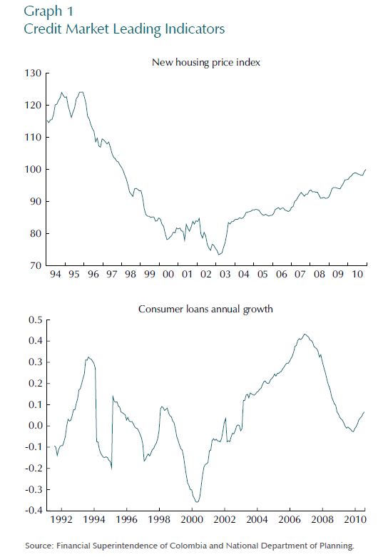
The behavior of consumer loans, presented in the lower panel in Graph 1, is somewhat related to the trends described above. This leading indicator showed a strong decrease between 1998 and 2000, and a marked acceleration every year thereafter. Following the tight credit conditions that followed the mortgage crisis of the late nineties, an important proportion of household expenditure was financed through consumer loans, which albeit representing higher interests, did not have the looming threat of losing the collateral backing the loan5. The peak of the new credit cycle was reached at the end of 2006, when consumer loans were growing at real annual rates of 45%. The Central Bank of Colombia decided to start raising interest rates in June,2006 and implemented marginal reserve requirements in 2007 with the goal of moderating the rapid growth of credit.
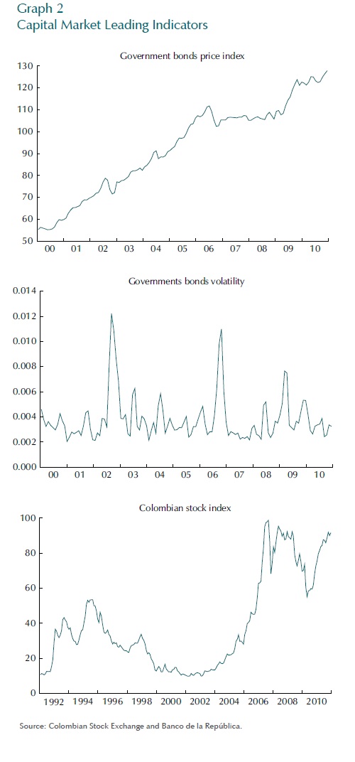
Similar to consumer credit and housing prices as leading indicators of their respective markets, indexes of government bonds and stocks are important for analyzing trends in capital markets. As shown in the upper row in Graph 2, it is noteworthy that the year 2002 was characterized as a period of high turbulence for government bonds in the secondary market. At the end of the nineties, with credit markets partially frozen, financial institutions began increasing their holdings of government bonds. Higher demand from credit institutions and institutional investors (such as pension and severance funds), coupled with lower interest rates, since the beginning of 2000 as the Central Bank looked to restore liquidity in the market, created an ideal atmosphere for growth in bond markets.
The increase of local interest rates during the period between July and September, 2002, as a consequence of the change in country risk, caused the prices of these securities to be adversely affected, market volatility to increase and financial institutions to experience big losses (Financial Stability Report, 2002). However, the impact of this episode on overall economic activity was of small magnitude, as the government bond market was still incipient in 20026.
But financial stress in the government bond market was not unique to the 2002 episode. Only four years later, in 2006, a period of high volatility affected the public debt market for a second time. According to the Financial Stability Report (2006), between February and June, 2006, the secondary market was characterized by an upward trend in the interest rates of government bonds which caused increases in the volatility of that market. This phenomena was linked to investors' expectations concerning the future path of monetary policy in the United States, which led them to liquidate their positions in emerging economies in the face of possible increments in foreign rates. Thus, the Colombian financial system faced significant valuation losses as a consequence of the large amount of government bonds held on their balance sheet.
In comparison to 2002, the magnitude of the bond market crisis in 2006 was significantly larger, as the total amount outstanding had more than doubled and the nonbanking sector held a bigger portion of these assets, in particular, pension and severance funds7. However, the impact on real activity was again minimized, not only due to the long-term investment horizon of pension and severance funds' investment portfolio, but also to the recomposition (loans vs government bonds) that took place on the banking sector's balance sheet. Following this period of financial distress, the market for government bonds has remained relatively stable in the most recent period. The Central Bank of Colombia started lowering interest rates at the end of 2008, and continued doing so until May, 2010. The recent low and stable level of interest rates has created favorable conditions in the government bond market and has helped consolidate the upward trend observed in prices since mid-2008.
The lower row of Graph 2 depicts the Colombian Stock Index for the period 1991-20108. During the nineties, many factors affected the Colombian stock market. In the first half of the decade, the ever-increasing capital inflows included considerable resources for investment in the stock market. Market capitalization grew during this period as a result of the larger number of firms listed on Colombian exchanges. In particular, market capitalization, as a percentage of GDP, grew from just 3% in 1990 to 19.3% in 19959. Nevertheless, at the beginning of 1995, Colombian stock market indicators started deteriorating âas a result of the crisis being faced by other emerging economies10â and eventually bottomed out during the country´s 1998-1999 recession period . Specifically, the Colombian Stock Index, which had grown at an average annual rate of 43% between 1992-1994, registered a significant contraction, growing at -2.5%, on average, between 1995-1999. Volatility also presented a noteworthy increase, particularly during the crisis of 1998-1999. While the first half of the nineties volatility was, on average, 1.5%, during the distress period, volatility mounted to 2.3%. The number of transactions in the market decreased drastically and many companies facing financial problems decided to stop trading on the market (Bernal and Ortega, 2004).
As can be observed in Graph 2, the merger of the three stock exchanges in Colombia during 2001, along with foreign investors renewed interest in emerging economies (as a response to the dot-com crisis in the United States) pushed the stock market into a new expansion period11. Similar to that for the growth period witnessed in the early nineties, the explanation for this phenomenon lies in the increased capital inflows into the Colombian economy and the increased demand for stocks from pension and severance funds, but also because of the modernization process of the Colombian Stock Exchange (Uribe, 2007).
During the last few years, the stock market has suffered from the effects of increased uncertainty in worldwide financial markets. The financial crisis in the United States played itself out through sharp falls in prices and higher volatility, which affected stock markets in both developed and emerging economies12. Additionally, higher risk aversion, after the collapse of Lehman Brothers, caused a decline in the "appetite" for riskier assets around the world. Colombia was no exception, as the volatility of its stock market returns between 2006-2008 was higher than for the whole period considered here (2% against 1.6%).
Since 2009, the Colombian economy has initiated an important recovery process in both credit and capital markets. The Colombian Stock Index began growing again and has recently shown important levels of appreciation as a consequence, at least partially, of the high demand for stocks in Colombia relative to the limited number of outstanding issues, the merger of the Colombian Stock Market with those of Peru and Chile and the modification of investment alternatives for pension and severance funds13.
IV. DATA AND METHODOLOGY
A. DATA AND INPUT FOR THE FCI
In selecting the variables to include in our index, we follow the spirit of Hatzius et al. (2010) and try to include financial variables from the most relevant markets in Colombia. Moreover, we include levels, growth rates, ratios, correlations and volatilities, so as to capture the different dynamics in the market and enhance the potential information regarding future outcomes embedded in our index. Still, there is usually a valid concern regarding the financial variables selected for the construction of the FCI. A question that seems to be relevant is: What is the motivation for including each of the variables in the index? (English et al., 2005). Schematically, we can classify the traditional variables included in a FCI and their importance in groups as follows:
•Interest rates: measure the cost of financing for firms and households.
•Exchange rates: affect GDP through net exports or can reflect the increased perception of risk from investors in a particular country.
•Interest rate spreads: changes in these variables might have two interpretations: It may reflect the higher demand for borrowing of firms to finance productive projects; at the same time, the unwillingness of banks to lend at previous rates due to constraint of funds. The first one would reveal that the economy will expand whereas the second would reflect a downturn (Swiston, 2008).
•Asset prices: determine the wealth of consumers and also the cost of capital of firms. Montagnoli and Napolitano (2006) provide three arguments on why asset prices are important in a financial index for monetary policy purposes.First, misalignments in asset prices can threaten financial stability. Second, they might affect the transmission of monetary policy through their effect on consumer wealth and the willingness of banks to lend, as they work as collateral for loans. Third, they contain future information about the economy, as they reflect expectations about inflation and general macroeconomic conditions.
•Credit aggregates: reflect both demand (economic outlook) and supply (not captured by interest rates) factors.
•Expected Inflation Surveys: Contain relevant information regarding the expected path of monetary policy.
In addition to the variables mentioned above, we also chose to include financial ratios from the banking and non-banking sectors. The reason for including the former is that these give a good indication of the build-up of risks in credit markets. The latter are included, since in Colombia these markets have grown vigorously in the last decade, and the size of their investment portfolios (and large concentration in local stocks and Government bonds) makes them a potential threat to financial and overall economic stability. On a final note, it is important to mention that, despite the importance that credit availability surveys have proven to have in the construction of FCIs (see Guichard and Turner, 2008; Hatzius et al., 2010; Swiston, 2008), we were not able to include such variables in our index. The Central Bank of Colombia currently applies a survey (on a quarterly basis) on credit availability at commercial banks, but this only began in 2008 and hence, the time series is still very short.
Furthermore, we would like to point out that, instead of the common practice found in the literature of including measures of level, slope and convexity in the spot curve, we use the aggregate government bond price index (IDXTES) proposed by Reveiz and León (2008). The reason for this choice is twofold. First, the price index should synthesize all the relevant information regarding the public debt market at all points in the curve. And second, as Cardozo and Rojas (2010) indicate, they have not found a statistically significant link between the common measures of level, slope and curvature of the spot curve and real activity for the case of Colombia14. Nonetheless, we include two measures of the slope of the government bond spot curve in our financial variables for completeness.
We use monthly data for the period comprised between July, 1991 - June, 2010. Not all our variables are available for the entire sample and so the nature of our dataset is an unbalanced panel.
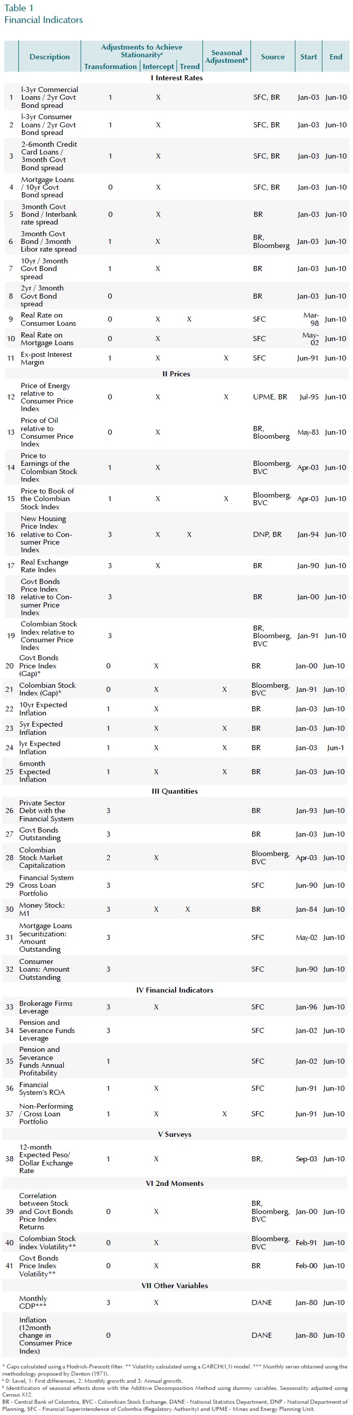
Following the general rule of thumb in the FCI construction literature, all our variables are in real terms and checked for seasonal effects and stationarity (and adjusted when necessary) and consequently standardized using each series' sample mean and standard deviation. The exact transformations conducted on each variable are found in Table 1. Our goal is akin to that of Hatzius et al. (2010), in that we wish to construct an FCI which is purged from the endogenous reflection in financial variables of past economic activity (i.e. we wish to capture pure financial shocks). Hence, we run a regression of each of our transformed variables against GDP and 12-month inflation (measured as the annual change in the Consumer Price Index), and use the residuals from these models to conduct our principal component analysis15. Indeed, from this point forward, the reader should be aware that when we make reference to our financial variables, we actually mean the residuals from the transformed variables.
The regressions estimated can be explicitly represented as:
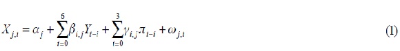
where  is the j-th financial indicator at time t,
  is annual GDP growth and
  is annual inflation. Ultimately, we are interested in the resulting
  , and assume we can decompose them as:
where  can be thought of as a vector of unobserved financial factors and
  captures idiosyncratic variations in which are assumed to be independent of both and . Assuming that the are uncorrelated across financial variables, implies that the vector of factors captures the co-movement in the financial indicator. We use least squares estimates of F (i.e. principal components), since these are accurate enough so as to be used in subsequent statistical analysis, including predictive regressions like the ones undertaken in what follows (see Bai and Ng, 2008; Eickmeier and Ziegler, 2008; Hatzius et al., 2010; Stock and Watson, 2006, 2010).
B. CONSTRUCTING THE FCI
As mentioned above, we use PCA to estimate the vector of unknown common factors F. Since our dataset is comprised of variables that begin at different points in time, and we wish to effectively exploit its unbalanced nature, we estimate the correlation matrix (on which we will perform the principal component analysis) without balancing the sample. Instead, we use pairwise deletion of missing values and thereby use the maximum number of observations for each (pairwise) calculation. Nonetheless, even though the estimation of the correlation matrix utilizes all available information, the calculation of its principal components is available only from the starting point of the balanced sample. Since we wish to obtain an index that goes back at least to the beginning of the nineties, we employ the following steps to construct our FCI back in time:
• We estimate the correlation matrix of our financial variables for the period between July, 1991 - June, 2010.
• Once our matrix is estimated, we perform PCA and obtain our principal components series starting on February 2004. We also record the factor loadings and percentage of the variance explained by each factor.
• We choose to work with the first 10 principal components, since these explain, roughly, 70% of the variance of the original dataset.
• Using the estimated factor loadings for the first 10 components, we "construct" loadings for the unbalanced part of our sample (i.e. July, 1991 - January 2004). In order to do so, we simply assume the following:
a) If there is no information available for the variable at time t, we assign a factor loading of 0.
b) If the variable is available we assign the factor loading originally calculated.
c) Since the new square of factor loadings will not add-up to 1 at each t, we rescale the square factor loadings to guarantee that this condition be met16.
d) Once our square loadings are rescaled, we calculate our new loadings and assume they have the same sign as the original ones.
• We now have a matrix of rescaled loadings for the period between July, 1991 and January 2004, for each of the first 10 principal components.
• Since a principal component can be expressed as the linear combination of each financial variable multiplied by its factor loading, we multiply the matrix of rescaled loadings by the transpose of the matrix which contains the financial variables to obtain our components for the unbalanced sub-sample.
The final step needed to construct a FCI is that of deciding how to combine the components in order to create a single indicator. There are at least two possibilities, and we explore them both. On the one hand, we simply choose to define the FCI as the first principal component, as proposed in Hatzius et al. (2010). The advantage of doing this is that the index will not lose tractability, and there is no need to make any further assumptions on how to combine the components arising from the PCA. On the other, we also work with a combination of the components in an attempt to construct a FCI that incorporates more information from the original dataset (i.e. that explains a larger portion of the dataset's variance). We again opt for a practicality argument and simply utilize the marginal explanatory power of each component in the cumulative variance to assign the relative weights of each component.
Once our FCIs are constructed, we decide to work with a moving average of the indicators17. The reason for this is twofold. First, it reduces some of the excessive short-term volatility that is inherent in financial series, and allows us to focus on the relevant common trends observed in the data. Second, in the spirit of Borio and Lowe (2003), when constructing leading and early-warning indicators, we are interested in persistent deviations in financial variables, since it is precisely periods of sustained imbalances that give rise to effects on real activity.
C. PURGING OF THE FINANCIAL VARIABLES' DATASET
Despite the fact that PCA allows us to summarize the information of a large number of variables into relatively few components, we are aware that the practicality of any indicator will be enhanced by identifying the fewest the number of variables needed to update it. Additionally, there is room to believe that many of our financial indicators may encompass the same relevant information for our FCI, and so we may purge our dataset in order to utilize only the most information-intensive variables. Nonetheless, we are aware that the loss of certain variables may generate a trade-off between predictive precision and parsimony. We do not believe the costs associated with this trade-off to be significant; so we carry out comparisons in our statistical tools between the FCIs built with all 41 variables and our purged FCIs for completeness.
In order to reduce the size of our dataset, the following criteria were used to identify disposable "candidates":
1) Relative weight in the first 2 principal components of less than 3%
2) Low predictive power of GDP growth using a VAR model
3) High correlation coefficient between financial variables
4) All variables with a correlation coefficient with GDP growth lower than 0.1
5) Low correlation of the lagged values of the variable (lags of 1st, 2nd and 3rd order) and GDP growth
6) Availability of information18
Once these filters were applied, we chose to remove all variables that met at least 3 of the 6 mentioned criteria or 2 of the first 3. The end result is a dataset which includes 21 variables19.
We now apply PCA to the new set of variables and reconstruct our FCIs using the same technique described in Section IV.B above20. The original FCIs, the purged FCIs, and GDP growth can be observed in Graph 3.
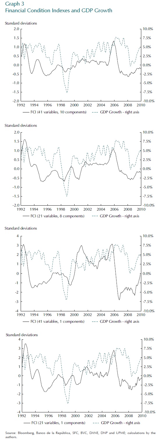
As can be seen, even when all the FCI's seem to capture the main fluctuations in GDP growth, the purged FCIs track GDP much closer than their 41 variable counterparts. This is an encouraging result in many ways. On the one hand, it suggests that, contrary to what we initially assumed, there seems to be no loss of relevant information when we trim the dataset. In fact, some of the variables removed might have been adding more noise than information. On the other hand, the joint movement in both financial conditions and real activity suggests that there may indeed be a relevant link between the two. Indeed, the 21 variable FCIs seem to anticipate some of the sharpest movements in GDP, such as the downturns in economic activity suffered in both 2008-2009 and the 1998-1999 mortgage crisis.
In addition, note that these strong downturns in the FCIs (and consequently in real activity) are generally preceded by periods characterized with sharp upturns, usually one or two years prior to the downfall. This is consistent with the idea that excessive and rapid growth in financial markets is usually a good indication of a profuse build-up of risks in the market, and that it is precisely such joint imbalances that we wish to monitor. Moreover, we conducted Granger causality tests and effectively found that the FCI causes GDP growth, though the inverse does not hold21. These results combined imply that our faith in the FCI as both a leading and early-warning indicator may not be unfounded.
V. RESULTS
A. OUT-OF-SAMPLE-PREDICTIONS
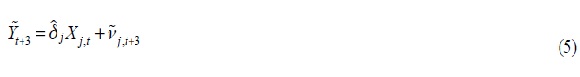
In order to test the predictive power of the FCIs we carry out several out-of-sample forecasting exercises. Here, we not only compare the performance of all FCIs against an AR model of GDP growth, but also test the predictive capacity of various leading indicators of Colombia's financial markets. Several forecasting horizons were considered (1-month, 3-month, 6-month and 12-month), but results here are only presented for a 3-month horizon, as these yielded the best results. The model used for forecasting can be explicitly represented as:
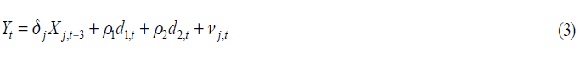
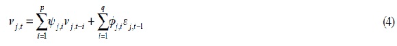
where is GDP growth, is the j â th financial variable considered, d1 and d2 are two dummy variables, which take a value of 1 after January, 1999 and January, 2002,respectively22 and vj,t is the residual term in equation (3). Instead of assuming that v is nothing more than a random noise process, we claim it incorporates relevant information regarding the dynamics of GDP growth, and hence explicitly model its behavior using an ARMA model23. Subsequently, we conduct a 3-month ahead forecast of v, so that at any point in time t, our forecast of GDP growth is simply given by:
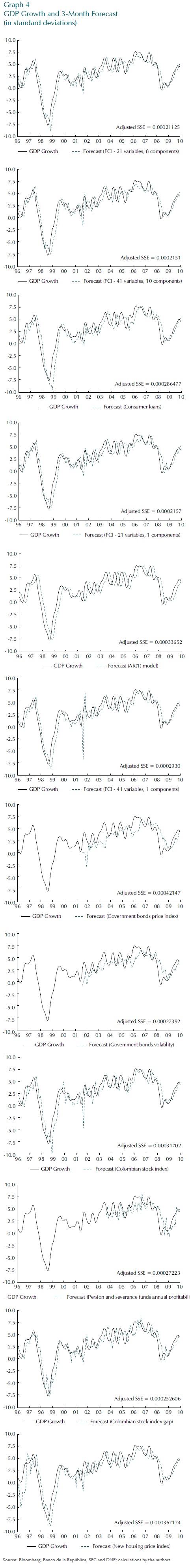
The out-of-sample exercises were done with an initial sample comprised of the period between July, 1991 - July ,1996, and therefore, our first forecast is October, 1996. Since not all variables have the same starting date, we compare between models using an Adjusted Sum of Squared Errors (Adjusted SSE)24.
Results for each of the indicators considered can be viewed in Graph 4. As can be seen, the prediction models which utilize the FCIs have the highest forecasting power, outperforming not only the leading indicators considered, but the autoregressive model of GDP growth as well.
Nonetheless, it is worth noting the impressive performance of univariate leading indicators, such as the Colombian Stock Index (both its annual growth and its gap), consumer loans and the volatility of government bonds. This result may be partly a consequence of the fact that Colombia's financial markets are still shallow and almost entirely comprised of government bonds, stocks and credit, so that proxies of each of these markets are expected to convey significant information on future economic activity. However, most of the leading indicators considered seem to do a decent job at predicting future economic performance, and the results are thereforeencouraging in providing both validity to the variables chosen in constructing the FCI and to the index itself as a leading indicator.
Therefore, we have that the FCI seems to be the best leading indicator here considered. Indeed, at a 3-month forecasting horizon, the FCI anticipated all significant downturns in economic activity. In other words, there is a tight link between financial conditions and economic activity, at least in the short-term. This result, significant on its own, poses a much more ambitious, and probably more relevant question from a policymaking perspective: With a longer horizon (i.e. one year) âAre significant and persistent deviations also indicative of future economic events? This is the question we now seek to formally answer.
1. Choosing the FCI
Results from the out-of-sample exercises suggested that all of our FCIs are ideal candidates as leading indicators of economic activity. Nonetheless, we wish to construct a unique FCI, and so are forced to choose between our 4 possibilities. We have decided to define the Financial Conditions Index for Colombia as the purged FCI constructed with the first principal component. The reasons for this choice should be readily apparent. First, the FCI constructed this way has the characteristic of tracking GDP appropriately, and more importantly, seems to anticipate periods of economic stress. Second, it does as well as the other indicators in the out-of-sample exercises conducted in Section V.A. Third, since it uses only the first principal component, there is no need to make additional assumptions on the most appropriate aggregation method between components. Additionally, it only uses 21 variables, so that updating this particular indicator is actually less time-consuming. Finally, and most importantly, by using only one principal component, the FCI constructed in this way has perfect tractability, and the policymaker can easily identify the specific market giving rise to a particular value of the index.
This last characteristic is extremely important in what follows, as we are effectively interested in constructing an early-warning indicator. Hence, it is ideal, from a supervisory perspective, to be able to trace a possible alert signal to the market(s) presenting the imbalance. Moreover, this allows our indicator to be comparable with other market-specific early-warning indicators in the spirit of those proposed by Kaminsky, Lizondo and Reinhart (1997), Kaminsky (1998), Kaminsky and Reinhart (1999) and Reinhart and Rogoff (2008).
The weight of each variable (i.e. the squared loading from the PCA) in the index is presented in Table 225.
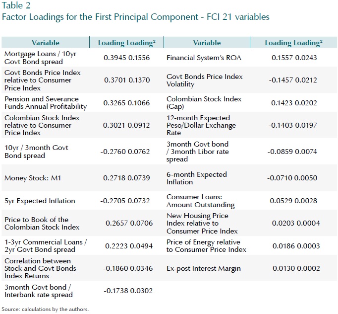
From Table 2 it is clear that the most relevant variables (in the balanced part of our sample) in the FCI include the spread between mortgage loans and the 10-year government bond rate, the price indices for both government debt and stocks, the profitability of pension and severance funds and the slope of the government bonds' spot curve. Together, these variables explain roughly 57% of the FCI. Furthermore, analyzing the factor loadings allows us to examine the effect that an increment in a given variable has on the index. In particular, we can see that increments in asset prices and higher levels of credit growth have a positive effect on financial conditions, whilst higher short-term rates in government bonds (relative to both Libor and the interbank rate) and a steeper spot curve adversely affect them. As expected, an increase in the correlation and volatility measures has a negative effect on the level of the index (i.e. loadings are negative). Interestingly, these results are consistent with those presented by Hatzius et al. (2010).
Additionally, we find that an increase in expectations regarding long-term inflation negatively affects financial conditions, presumably due to the increment in the interest rates that they trigger. These expectations are reflected in the inflation surveys and the slope of the bond yield curve. Moreover, episodes of high market liquidity, reflected in higher quantities of monetary aggregates (M1) and lower spreads of interbank rates with respect to government bond yields, are related to higher levels of our FCI.
On a final note, it is remarkable that the profitability of pension and severance funds has such a high weight in our FCI. The growing importance of these institutions in local financial markets, along with the concentration of their investment portfolios in local assets (especially government bonds and stocks) can help explain this outcome.
B. EARLY-WARNING INDICATOR
An indicator such as the FCI, which collects information regarding various financial variables, can be used as a tool for macroprudential policy. In fact, these kinds of indicators should be a source of relevant information concerning future episodes of distress. By carefully monitoring the evolution within these indexes, the institutions in charge of prudential policy can act, or at least be prepared in advance, to face macro-financial disturbances. Following this idea, the purpose of this section is to evaluate our FCI as an early-warning indicator.
Most of the past scenarios of economic stress in Colombia have been preceded by scenarios characterized by extraordinary behavior in some financial indicators. This characteristic can be, at least partially, explained by the waves of optimism in specific markets that tend to disproportionately increase relative prices. For instance, the financial crisis at the end of the nineties was preceded by an important increase in both mortgage and stock prices26. As a result, disproportionate behavior in terms of both growth and level of the FCI should be used as signals of possible subsequent scenarios of financial distress.
In order to determine moments of unusual levels and growth of financial conditions, we carry out two exercises. The first one is designed to determine uncommon deviations in terms of the level of financial conditions in Colombia. The second exercise identifies scenarios in which the growth of our FCI was especially high. The main purpose of both exercises is to evaluate the relationship between these unusual deviations and subsequent scenarios of stress.
Two reasonable concerns when interpreting the results of these exercises are readily apparent. On the one hand, is the choice of the threshold value that defines such unusual deviations, since the results will undoubtedly be affected by it. On the other, is the fact that we wish to capture persistent deviations, and not simply periods of excessive short-term volatility.
In addressing the first of these issues, note that although highly sophisticated methods could have been used in order to determine the optimal threshold values, the approach followed here is more practical in nature and follows the spirit of the early-warning indicators developed by Borio and Lowe (2003). In this sense, we evaluated a range of relevant threshold values, rather than one value alone, and then opted for a specific value using two criteria:
1) That the indicator surpassed the threshold (i.e. generated a signal) for the two periods of significant economic downturn identified in Section IV.C above; namely, 1998-1999 and 2008-2009.
2) That the number of false signals was minimized.
Concerning the duration of the imbalances to be considered persistent, we chose to identify a signal when the FCI is above the chosen threshold for one period. The rationale behind this is that the FCI is constructed as a 12-month moving average of financial conditions. Therefore, there is a high likelihood that an unusual one-period deviation in the FCI is already capturing an accumulation of imbalances rather than an extreme outlier.
1. Early-Warning Using Levels
First, we study the level of the FCI using a time series analysis approach. The basic idea is to identify special deviations of the historical level of the FCI relative to some benchmark value. By doing so, we can identify whether such special deviations of financial conditions can be interpreted as an early-warning indicator. In order to develop this analysis, we do a time series decomposition of the FCI using the Hodrick-Prescott Filter. This decomposition allows us to discriminate the cyclical behavior from the trend component of the series. Hence, a special deviation of the FCI is defined when the index reaches a level higher than the sum of the long-term component and one and a half standard deviations of the cyclical component of the index.
Following the previous definition, the FCI has presented relatively high deviations during five episodes over our period of analysis (see Graph 5): November 1992 - April 1993 (Period 1), September 1994 - December 1994 (Period 2), October 1997 - December 1997 (Period 3), January 2002 - March 2002 (Period 4) and September 2005 - August 2006 (Period 5). It is quite important to notice that most of the periods of special deviation of the FCI under our definition are followed by either scenarios of economic slowdown or financial stress27. Period 2 was followed by a deceleration of economic activity in 199628. Following this same pattern, Period 3 was followed, with a one year lag (the end of 1998), by the most important crisis that the Colombian economy has suffered in the last two decades29. Period 4 is located six months prior to August 2002, which, as was mentioned in Section III, was a turbulent time in the secondary market for government bonds.
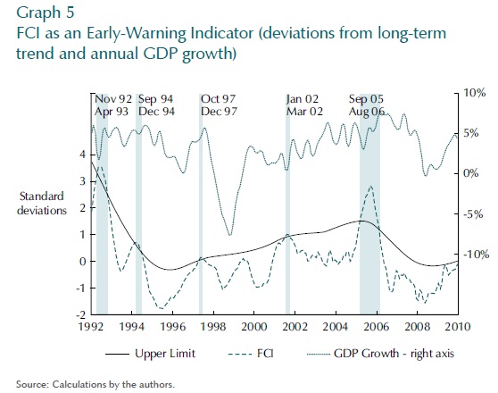
Finally, Period 5 begins four months prior to a period of special losses in the public debt market and continues presenting a possible imbalance two years prior to the economic deceleration period of the last quarter of 2008 and first half of 2009. Therefore, it seems plausible to suggest that the FCI is capturing a dual effect. On the one hand, there may genuinely be a reflection of the imbalances that had started to build-up in financial markets as a result, among others, of high levels of global liquidity and lower risk aversion, leading to excessive risk-taking by market participants. Additionally, and very relevant in the case of Colombia, the surge in the level of the FCI may be a direct consequence of the high levels of volatility experienced in the government bond market,as well as the surge in the consumer loan portfolio and in stock prices witnessed in this period, since these three variables are key components of the FCI. As mentioned in Section III, the market for government bonds went through a period of increased uncertainty during most of 2006. Specifically, for the period between February and August 2006, these bonds doubled their average historical monthly volatility, reaching 0.6%. Likewise, consumer loans and the Colombian Stock Index registered an average annual expansion of 39.2% and 56% during this period, while their historical averages reached no more than 5.9% and 10%, respectively.
2. Early-Warning Using Absolute Changes
As was mentioned above, the second exercise is designed to identify how scenarios of rapid change in our FCI can anticipate episodes of stress and economic deceleration30. We defined a moment of special change (i.e. a signal) using the 85th percentile of the semestrial shifts of the FCI. The semestrial absolute change equivalent to this percentile is 1.4.
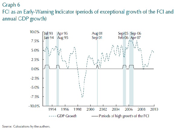
According to this definition, there have been five scenarios or signals of specially high change in the FCI (see Graph 6). Scenario 1 was registered between July 1993 - January 199431. The second period (Scenario 2) is located between April and August 1995. As we mentioned before, in 1996, the Colombian economy went through a phase of economic slowdown. The third signal (Scenario 3) occurs between August and September 2001, practically one year prior to the stress scenario observed in government bond markets. As can be readily noticed, these signals are also observed in the exercises carried out in Section V.B.132.
The dual effect that was mentioned for Period 5 in the early-warning exercises performed above, seems to be naturally reflected in the exercises using absolute changes.Scenario 4, which is located between September 2005 and February 2006, anticipates a period of special losses in the public debt market. Despite the fact that, unlike the 2002 stress scenario, the market for government bonds had deepened, there seems to be no significant effects on the real economy either. Nonetheless, this seems to be closely related to the duration of the period of increased uncertainty relative to the investment horizon of the bond holders. On the one hand, pension and severance funds, one of the major holders of government bonds at the time, had significantly long investment horizons, so that a 3-month period of volatility and falling prices would undoubtedly affect their tri-annual profitability measures (albeit marginally), but would not induce massive fire-sales or significant wealth losses for the individuals that invest in them33. The same is true for many other institutional and individual investors which see government bonds as safe (i.e. risk-free), long-term assets. Moreover, commercial banks, which also have considerable holdings of these assets, did not suffer significant losses as they undertook a massive asset substitution strategy34. The fifth signal (Scenario 5) which is located between September 2006 - August 2007, was followed by a period of important economic deceleration in the last quarter of 2008 and first half of 2009, in no small part due to the increased uncertainty in markets as the global financial crisis unfolded.
On a final note, we would like to emphasize the fact that defining signals through rapid absolute changes in the FCI comes at a cost. Namely, that imbalances that build-up slowly through an extended period of time are not captured by this indicator. Such is the case of the mortgage crisis of 98-99, whose imbalances began to accumulate starting in the first half of the nineteen-nineties. This result is a clear indication that both indicators should be used as complementary tools for macroprudential purposes.
In general, we are aware that some of the signals presented by both our early-warningindicators (i.e. using levels and absolute changes), identify periods that are not followed by episodes of economic slowdown. However, it is important to highlight that these signals are not necessarily wrong because they are not predicting scenarios of economic deceleration. On the contrary, the fact that these signals are located in periods of significant financial stress that were not accompanied by an episode of economic slowdown may be due to other idiosyncratic factors that do not invalidate the relevance of such signals for policymakers. More specifically, we believe there is a combination of two factors. In the first place, that the imbalances captured by these periods occur in markets that are not yet deep enough to have significant direct impacts on real activity. Secondly, that these periods of extreme volatility are shortlived relative to the investment horizon of the agents it most affects.
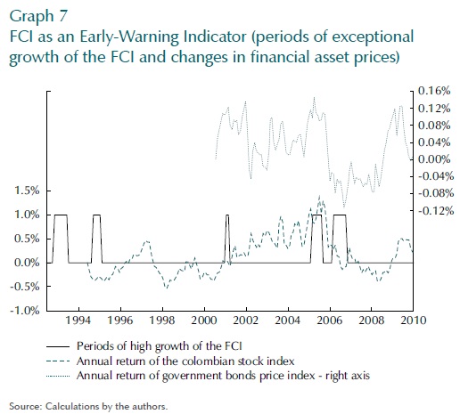
In order to elaborate the argument, Graph 7 illustrates the link between periods of rapid absolute change of the FCI and subsequent periods of low historical returns on the main financial asset prices in Colombia. From the graph, it is clear that the earlywarning signals are effectively contemporaneous to periods of accelerated changes in both stock and bond prices, which could effectively be early symptoms of excessive risk-taking.
Overall, we believe that as stock and bond markets become deeper and more complex, periods of stress in these markets that do not result in downturns in real activity will be less likely. A stronger development in these markets will ultimately lead to tighter interconnections with other markets, thus elevating the likelihood of a more direct impact on the real economy through contagion effects. This is the main reason why we feel comfortable with the early-warning indicators effectively anticipating scenarios of financial stress in these markets, and find it a desirable quality from a forward-looking policy perspective.
VI. CONCLUINDG REMARKS
The last few decades have seen an enormous growth in financial markets. Investors around the world now have more investment vehicles and possibilities than ever before. The latter has allowed for a smoother flow of funds and a more efficient allocation of resources, with agents choosing products that better suit their individual risk appetites. However, this proliferation of financial innovation has come at the cost of more opaque financial products and complex interactions between markets. From a policy perspective this poses a great challenge, as the growth of financial markets implies both a possible stronger impact on the business cycle and a more complicated approach to adequate supervision.
This paper attempts to construct a simple, yet effective, macroprudential tool for policymakers. By integrating the joint behavior of the most relevant financial variables in Colombia into a single indicator, we hope to synthesize the information embedded in financial variables regarding possible future economic outcomes. To do this, we apply PCA on the correlation matrix of 21 financial variables that span the most significant markets of the financial system and use a 12-month moving average of the resulting index to carry out our empirical exercises. Our faith in such an ambitious endeavor stems from the fact that several authors have documented the close link that exists between periods of joint imbalances in financial markets and subsequent scenarios of economic stress (Bernanke et al., 1998; Borio and Lowe, 2003; Collyns and Senhadjy, 2003).
We find that our FCI not only performs better as a leading indicator of 3-monthahead real activity than other individual financial variables, but also than an autoregressive model of GDP growth. This result is encouraging in that it confirms the intuition that financial variables, and more specifically joint movements in the latter, effectively contain relevant information regarding future outcomes in real activity. Based on these results, we decided to undertake a more ambitious, and possibly more important, task: to test the usefulness of the FCI as an early-warning indicator.
We find that the FCI can indeed be used as an early-warning indicator, and therefore represents a useful instrument for financial stability purposes. Using criteria that consider unusually high deviations both in terms of levels and absolute changes of the FCI to define our thresholds, we find that periods which activate our signals are highly correlated with subsequent scenarios of financial distress and/or episodes of economic deceleration. Despite the fact that we have some signals that are not followed by economic downturn, we feel optimistic that these periods indeed correspond to scenarios of excessive volatility in financial markets. As the latter continue deepening in Colombia, their direct and indirect effects on real activity should be magnified, and thus we feel comfortable with the early-warning indicators readily anticipating scenarios of stress in these markets. In fact, from a macroprudential perspective, we find this characteristic advantageous, as it gives authorities time to act, or at least be better prepared, before such imbalances result in a period of financial distress that could potentially affect the real economy.
The recent trend in regulatory and supervisory reform, led by Basel III and the ongoing financial reform in the United States, is to move towards a more systemic and macroprudential framework. In this spirit, the development of tools such as the earlywarning indicator attempted herein, is a first step towards building a more sound and resilient financial system. However, the construction of decent early-warning mechanisms by themselves should not be the ultimate goal of policymakers, since acting as a safety-net every time financial markets experience excessive risk-taking attitudes may endogenously create the incentives for such behavior (i.e. moral hazard). On the contrary, these instruments should be used to alert policymakers on the markets that are most prone to suffer financial distress periods. By fulfilling this role, such signals would give clearer direction to efforts focused on improving the proper functioning of such markets and the promotion of private solutions to possible imbalances.
Comentarios
1 Goodhart (2001) and Goodhart and Hofmann (2001) expose this kind of transmission mechanism clearly, and justify why central banks should be concerned with asset prices when targeting inflation.
2 The list of variables included in our index and the justification for their inclusion is presented in Section IV below.
3 Goodhart and Hofmann (2001) also mention model dependence of the derived weights as a potential caveat when estimating FCIs. Nonetheless, we feel that this is a criticism that applies to any kind of empirical analysis, and so we omit it from the discussion that follows.
4 Other variables included are corporate bond spreads, equity prices, real exchange rates and credit aggregates.
5 In fact, commercial and mortgage loans only perceived positive growth rates in 2003 and 2005, respectively.
6 The total amount outstanding of government bonds in 2002 was just COP$50 billion (total credit was also equal to COP$50 billion) of which public entities held 20%, commercial banks 17.8%, pension funds 8.8% and brokerage firms 1.2%.
7 In 2006, the total amount outstanding was COP$115 billion (total credit, COP$90 billion) with commercial banks holding 18.8%, pension funds 22.2% and brokerage firms 0.4%.
8 The Colombian Stock Index (IGBC) is calculated by the Colombian Stock Exchange (BVC). In July, 2001, the 3 Stock Exchanges operating in Colombia (Bogotá, Medellín and Occidente) merged into the Colombian Stock Exchange. The historical price index series was constructed by the BVC.
9 Other factors contributing to the observed growth were the positive expectations regarding emerging markets and the creation of the pension and severance funds´ system in Colombia in 1993.
10 Mexican crisis in 1995, Asian crisis in 1997, and Russian crisis in 1998.
11 Between 2000 and 2005, market capitalization as a share of GDP grew 261%, even though the number of firms listed fell from 190 to 94 in the same period.
12 Clavijo and González (2009).
13 Private investors will now be able to choose their portfolio based on their risk profile. The high-risk category will have higher ceilings on the portion of the investments that can be allocated to local stocks than is currently allowed (i.e. from 35% to 45%).
14 The authors, however, do find a significant relationship between some of these variables and inflation.
15 A monthly series of GDP was obtained using the methodology proposed by Denton (1971).
16 To rescale we simply divide the square factor loading by the sum of the square factor loadings of the variables available at each t.
17 Specifically, we work with a 12-month moving average. Other orders were considered and the choice between them was based on the relative ability of each to forecast GDP growth using insample predictions.
18 In this respect we have two different criteria. Most important is whether the information for the financial variable is effectively available before GDP is made public. Additionally, we try to choose variables that have an adequate number of available data points, so as to make the estimation of our parameters more consistent.
19 The 21 variables used for the purged FCIs are those whose number is circled on Table 1.
20 The only differences in the construction of both indexes is that, in this case, the matrix of rescaled loadings is for the period July, 1991 - September, 2003; the unbalanced part of the sample. In addition, the FCI that is constructed as a linear combination of the components utilizes the first 8 principal components.
21 The latter result is expected since we explicitly controlled for the problem of endogeneity.
22 The inclusion of the dummy variables is based on Chow Tests for structural break conducted on the GDP growth series.
23 We use the same model specification for v for all the financial variables considered. In the AR model of GDP growth v is treated as a traditional error term. The order of the ARMA model is chosen using the Box-Jenkins methodology.
24 We perform a t-test in order to compare the relative performance among variables in terms of predictability. Test results are available upon request.
25 Recall that the loadings change through time to account for the fact that our sample is unbalanced. Therefore, the loadings presented correspond to those of the balanced sample, that is October, 2003 - June, 2010. Moreover, the squared factor loading is related to the explanatory power of each variable, since the sum of the squared loadings must be equal to 1.
26 The average real annual growth of the Colombian Stock Index during 1997, the year previous to the financial crisis, was 24.88%, which is highly above the historical average of 13.3%. Moreover, housing prices, measured by the New Housing Price Index, reached historical highs in the years previous to the 98-99 crisis. While during the period 1994-1997 housing prices were, on average, 1.6 standard deviations above their historical mean, the ten-year period that followed the financial crisis was -0.48 standard deviations below, on average.
27 There does not seem to be a relevant period of either economic slowdown or financial distress following Period 1. Thus, we consider this signal a s a false alarm.
28 In the period from 1990 to 1995 the average growth of GDP was 4.45%. In 1996, average growth suffered an important deceleration and was a mild 1.87%. The latter was due to an important contraction in Venezuela's demand (Colombia's second largest commercial partner) and supply shocks to the coffee sector caused by adverse weather conditions. Additionally, during the first half of the nineties Colombia's local interest rates were at extraordinarily high levels (average lending rates between 1990-1996 surpassed 40% whilst their 2000-2010 average reached 16.1%), significantly increasing the cost of capital for firms and specifically trumping the dynamics of two key industries for economic growth: the manufacturing and construction sectors.
29 The Colombian economy contracted at an average rate of -4.4% in the period from August 1998 to December 1999. This is remarkable if one keeps in mind that for the other two scenarios of economic downturn identified (i.e. 1996; and October, 2008 - June, 2009), GDP grew at an average rate of 1.87% and -0.7%, respectively.
30 We define the absolute change as 
31 In order to distinguish the periods where our indicators signal an alert, we define those of the first exercise as Periods and those of the latter as Scenarios.
32 Moreover, just as in the prior exercise, the first signal is deemed as a false alarm.
33 As of August 2006 only 20,000 people out of 6,799,000 affiliates were receiving a pension from their private funds. By November 2010 these numbers were 42,000 and 9,183,078, respectively. A significant increment in the number of retired individuals is not expected until around 2030, since the bulk of affiliates are concentrated in the 30-45 year-old range (www.superfinanciera.gov.co).
34 In a 3-month period (between March and June 2006), commercial banks sold close to COP $665 b in government bonds and began an aggressive loan portfolio expansion which resulted in the credit boom experienced in late 2006 and 2007.
REFERENCES
1. Bai, J.; Ng, S. "Large Dimensional Factor Analysis", Foundations and Trends in Econometrics, vol. 3, num. 2, pp. 89-163, 2008. [ Links ]
2. Banco de la República (BR).Survey on expected peso - dollar Exchange rate, government bonds price index, several years. [ Links ]
3. Banco de la República. "Reporte de Mercados Financieros", Financial Markets Report First Quarter 2010, Central Bank of Colombia, 2010. [ Links ]
4. Bernal, H.; Ortega, B. "Se ha desarrollado el mercado secundario de acciones colombiano durante el período 1988-2002?" Post-graduate monograph, Departamento de Economía, Universidad Externado de Colombia, 2004. [ Links ]
5. Bernanke, B.; Gertler, M. "Inside the Black Box: The Credit Channel of Monetary Transmission", Journal of Economic Perspective, vol. 9, num. 4, pp. 27-48, 1995. [ Links ]
6. Bernanke, B.; Gertler, M.; Gilchrist, S. (1998). "The Financial Accelerator in a Quantitative Business Cycle Framework", NBER Working Paper, num. 6455, Cambridge, MA. [ Links ]
7. Bloomberg . www.bloomberg.com. Statistics on Colombian stock index, Price to earnings , Price to book, price of oil, libor, several years. [ Links ]
8. Bolsa de Valores de Colombia (BVC). www.bvc.com.co. Statistics Price to earnings , Price to book, Colombian stock index, Colombian Stock Market Capitalization, several years. [ Links ]
9. Borio, C.; Drehmann, M. "Towards an Operational Framework for Financial Stability: âFuzzy' Measurement and its Consequences", BIS Working Papers, No 284. Bank for International Settlements, 2009. [ Links ]
10. Borio, C.; Lowe, P. "Asset Prices, Financial and Monetary Stability: Exploring the Nexus", paper presented at the BIS Conference on \ Changes in Risk Through Time: Measurement and Policy Options, BIS Working Papers, num. 114, Basel, 2002. [ Links ]
11. Borio, C.; Lowe, P. "Imbalances or âBubbles?' Implications for Monetary and Financial Stability", in C. Hunter, G. Kaufman and M. Pomerleano (Eds.), Asset Price Bubbles: The Implications for Monetary, Regulatory and International Policies (pp. 247-270), Cambridge, MA, MIT Press, 2003. [ Links ]
12. Cardozo, P.; Rojas, S. "Analysis of Latin American Spot Curves: What Can We Get From the Colombian Spot Curve?", mimeograph,Banco de la República de Colombia, 2010. [ Links ]
13. Clavijo, S.; González, A. "Mercados de renta variable y crisis internacional", Enfoque, Mercado de Capitales, núm. 33, ANIF, 2009. [ Links ]
14. Collyns, C.; Senhadjy, A. "Lending Booms, Real Estate Prices and the Asian Crisis", in C. Hunter, G. Kaufman and M. Pomerleano (Eds.), Asset Price Bubbles: The Implications for Monetary, Regulatory and International Policies (pp. 101-125), Cambridge, MA, MIT Press, 2003. [ Links ]
15. Denton, F. "Adjustment of Monthly or Quarterly Series to Annual Total: An Approach based on Quadratic Minimization", Journal of the American Statistical Association, vol. 66, pp. 92-102, 1971. [ Links ]
16.Departamento Nacional de Planeación (DNP).www.dnp.gov.co.Statistics Housing Price Index, several years. [ Links ]
17. Departamento Administrativo Nacional de Estadística (DANE). www.dane.gov.co. Statistics Gross Domestic Product, Consumer Price Index, several years. [ Links ]
18. Eickmeier, S.; Ziegler, C. "How Successful are Dynamic Factor Models at Forecasting Output and Ination? A Meta-Analytic Approach", Journal of Forecasting, vol. 27, num. 3, pp. 237-265, 2008. [ Links ]
19. Eika, K. H.; Ericsson, N. R.; Nymoen, R. "Hazards in Implementing a Monetary Conditions Index", Oxford Bulletin of Economics and Statistics, vol. 58, num. 4, pp. 765-790, 1996. [ Links ]
20. English, W.; Tsatsaronis, K.; Zoli, E. "Assessing the Predictive Power of Measures of Financial Conditions for Macroeconomic Variables", in Investigating the Relationship Between the Financial and the Real Economy, BIS papers, num. 22, 2005. [ Links ]
21. Financial Stability Report. Banco de la República de Colombia, December, 2002. [ Links ]
22. Financial Stability Report. Banco de la República de Colombia, September, 2006. [ Links ]
23. Financial Stability Report. Banco de la República de Colombia, March, 2007. [ Links ]
24. Gómez, E.; Rozo, S. "Beyond Bubbles: The Role of Asset Prices in Early-Warning Indicators", Ensayos sobre Política Económica, vol. 26, num. 56, pp. 114-148. [ Links ]
25. Goodhart, C. "What Weight Should Be Given to Asset Prices in the Measurement of Inflation?" Economic Journal, vol. 111, pp. F336-357, 2001. [ Links ]
26. Goodhart, C.; Hofmann, B. "Asset Prices, Financial Conditions and the Transmission of Monetary Policy", paper prepared for the conference on "Asset Prices, Exchange Rates, and Monetary Policy", Stanford University, March 2-3, 2001. [ Links ]
27. Guichard, S.; Turner, D. "Quantifying the Effect of Financial Conditions on US Activity", Working Papers, num. 635, OECD Publishing, Economics Department, 2008. [ Links ]
28. Hatzius, J.; Hooper, P.; Mishkin, F. S.; Schoenholtz, K. L.; Watson, M. W. "Financial Conditions Indexes: A Fresh Look After the Financial Crisis", Working Paper, num. 16150, National Bureau of Economic Research, 2010. [ Links ]
29. Kaminsky, G.; Lizondo, S.; Reinhart, C. "Leading Indicators of Currency Crises. Policy Research", Working Paper, num. 1852, The World Bank, 1997. [ Links ]
30. Kaminsky, G. "Currency and Banking Crises: A Composite Leading Indicator", Working Paper, Board of Governors of the Federal Reserve System, 1998. [ Links ]
31. Kaminsky, G.; Reinhart, C. "The Twin Crises: The Causes of Banking and Balance-of-Payments Problems", American Economic Review, vol. 89, num. 3, pp. 473-500, 1999. [ Links ]
32. Mayes, D.; Virén, M. "Financial Conditions Indexes", Discussion Papers, Bank of Finland, 2001. [ Links ]
33. Montagnoli, A.; Napolitano, O. "Financial Condition Index and Interest Rate Settings: A Comparative Analysis", Discussion Paper, num. 2, Department of Economic Studies, University of Naples "Parthenope", 2006. [ Links ]
34. Reinhart, C.; Rogoff, K. "This Time is Different: A Panoramic View of Eight Centuries of Financial Crises", NBER Working Paper, num. 13882, p. 160, 232, 280, 290, 371, 384, 2008. [ Links ]
35. Reveiz, A.; León, C. "Índice representativo del mercado de deuda pública interna: IDXTES", Borradores de Economía, núm. 488, Banco de la República de Colombia, 2008. [ Links ]
36. Stock, J.; Watson, M. "Macroeconomic Forecasting Using Diffusion Indexes", Journal of Business and Economic Statistics, vol. 20, num. 2, 2002. [ Links ]
37. Stock, J.; Watson, M. "Forecasting With Many Predictors", in G. Elliot, C. Granger, and A. Timmermann (Eds.), Handbook of Economic Forecasting (Ch. 6. pp. 515-554), Elsevier, 2006. Amsterdam: North Holland. [ Links ]
38. Stock, J.; Watson, M. "Dynamic Factor Models", in M. Clements and D. Hendry (Eds.), Oxford Handbook of Economic Forecasting, Oxford, Oxford University Press, 2010. [ Links ]
39. Superintendencia Financiera de Colombia (SFC) . Statistics on Interest rates, Financial System Gross Loan Portfolio, Mortgage Loans Securitization (Amount Outstanding), Consumer Loans (Amount Outstanding), and financial indicators , several years . [ Links ]
40. Swiston, A. "A U.S. Financial Conditions Index: Putting Credit Where Credit is Due", Working Paper, num. 08/161, International Monetary Fund, 2008. [ Links ]
41. Tenjo, F.; Lopez, M. "Early Warning Indicators for Latin America", Ensayos sobre Política Económica, vol. 28, num. 63, pp. 232-259, 2010. [ Links ]
42. Tenjo, F.; Lopez, E. "Burbuja y estancamiento del crédito en Colombia", Borradores de Economía, núm. 215, Banco de la República de Colombia, 2002. [ Links ]
43. Unidad de Planeación Minero Energética (UPME). www.upme.gov.co. Statistics price of energy, several years. [ Links ]
44. Uribe, J. M. "Caracterización del mercado accionario colombiano, 2001-2006: un análisis comparativo", Borradores de Economía, núm. 456, Banco de la República de Colombia, 2007. [ Links ]
45. Villar, L.; Salamanca, D.; Murcia, A. "Crédito, represión financiera y flujos de capitales en Colombia: 1974-2003", Revista Desarrollo y Sociedad, Universidad de los Andes-CEDE, 2005, pp. 167-209. [ Links ]
46. Zarnowitz, V. "Composite Indexes of Leading, Coincident and Lagging Indicators", in V. Zarnowitz (Ed.), Business Cycles: Theory, History, Indicators and Forecasting (Ch. 11, pp. 316-356), Chicago, University of Chicago Press, 1992. [ Links ]
