Una herramienta para el análisis de la política aplicada a las necesidades de Colombia: descripción del modelo Patacon*

Uma ferramenta para a análise da política às necessidades da Colômbia: Descrição do modelo Patacon*

Andrés González
Lavan Mahadeva
Juan D. Prada
Diego Rodríguez

*This work represents the sole opinions of the authors and not the Board members of the Banco de la República of Colombia. We wish to thank Lawrence Christiano, Fabio Canova, Douglas Laxton, Hernando Vargas, Camilo Tovar, Franz Hamann, Pietro Bonaldi, Christian Bustamante, Sergio Ocampo, Juan C. Parra, Julián Pérez, Luis E. Rojas and the participants of the 2008 Central Bank Workshop on Macroeconomic Modelling for their very helpful comments and discussions. A detailed version of the document with the derivations of each one of the agents' problems, the set of equations, variables and parameters of the model is available at http://www.banrep. gov.co/docum/ftp/borra656.pdf.

The authors are respectively: Director, Department of Macroeconomic Models, Banco de la República; Senior Research Fellow, Oxford Institute for Energy Studies, Oxford University; Ph. D. student in Economics at the Northwestern University; and head of Macroeconomic Models Unit, Department of Macroeconomic Models, Banco de la República.

E-mail: agonzago@banrep.gov.co; lavan.mahadeva@bankofengland.co.uk; juanprada2013@u.northwestern.edu; drodrigu@banrep.gov.co.

Document received: 25 May 2011; final version accepted: 30 August 2011.

In this document we lay out the microeconomic foundations of a dynamic stochastic general equilibrium model, called Policy Analysis Tool Applied to Colombian Needs (PATACON), designed as a forecast tool and as a guide to advise monetary policy authorities in Colombia. In companion documents we present other aspects of the model, including the estimation of the parameters that affect dynamics and impulse response functions.

JEL classification: E32, E52, F41.

Keywords: monetary policy, DSGE, small open economy.

En este artículo describimos los fundamentos microeconómicos de un modelo de equilibrio general dinámico y estocástico llamado "herramienta para el análisis de la política aplicada a las necesidades de Colombia" (Patacon, por su sigla en inglés); una herramienta predictiva que se utiliza como guía para el diseño de las políticas económicas de Colombia. En documentos complementarios describimos aspectos adicionales de este modelo, incluyendo el cálculo de los parámetros que afectan las funciones de dinámica y de impulso-respuesta.

Clasificación JEL: E32, E52, F41.

Palabras clave: política monetaria, DSGE, economía pequeña y abierta.

Neste artigo, descrevemos os fundamentos microeconômicos de um modelo de equilíbrio geral dinâmico e estocástico chamado "ferramenta para a análise da política às necessidades da Colômbia" (Patacon, por sua sigla em inglês); uma ferramenta projetada para ser preditiva e utilizada como guia para as autoridades em políticas econômicas da Colômbia. Além disso, descrevemos aspectos adicionais deste modelo, incluindo o cálculo dos parâmetros que afetam as funções de dinâmica e de resposta ao impulso.

Classificação JEL: E32, E52, F41.

Palavras chave: política monetária, DSGE, economia pequena e aberta.

I. Introduction

In this document we present a dynamic stochastic general equilibrium model designed to forecast and to provide guidance for monetary policy in Colombia. We call the model Policy Analysis Tool Applied to Colombian Needs (PATACON). The model is similar to models used in other small open economies. For example, the Riksbank, the central Bank of Sweden, uses the model by Christiano, Trabandt and Walentin (2007). The Bank of Spain uses MEDEA, a DSGE model by Burriel and Rubio-Ramirez (2009). The Bank of Norway and the Bank of Canada constitute other examples.

PATACON is a New Keynesian model constructed on top of a neoclassical growth model in which economic agents optimize the use of their resources over time. The source of growth is exogenous and depends on technological change and the rate of population growth. Following the work of Christiano, Eichenbaum and Evans (2005) and Smets and Wouters (2007), this model has been augmented to match the data with features such as sticky nominal wages and prices, as well as real rigidities such as habit in consumption, adjustment costs in investment, variable capital utilization and endogenous capital depreciation.

As its name implies, PATACON is tailored to match particular Colombian economic circumstances. For instance, Colombia is a net international borrower and consequently, it is influenced by changes in world capital markets. The model has, therefore, to allow for external world interest rates and perceptions of Colombian risk to affect domestic developments. The first effect is captured by a world interest rate, the second by a sustainable ratio of net foreign assets to GDP that can be altered along with perceptions of risk. World demand also matters, through export demand. Therefore, the external factors that have been important for the Colombian macroeconomic outlook are present in the model.

Although Colombia is not very open to trade¹,world prices do matter for GDP and inflation. This is probably because imports are complementary in domestic production and consumption. That said, the import price is affected by commercialization within domestic borders. In brief, this calls for a model with different types of imported input capital, raw materials and consumption products, each of which can be complementary in intermediate or final consumption with domestically produced inputs. Naturally, there should be a role for domestic margins in affecting the pass- through, as suggested in studies such as those by Parra (2010), or González, Rincón and Rodríguez (2010). Another channel by which world prices matter is through export prices and so revenues, a recurrent theme of Colombia's economic history (Mahadeva and Gómez, 2010).

The evidence reported in Julio (2010); Julio, Zárate and Hernández (2010); Iregui, Melo and Ramírez (2009); Misas, López and Parra (2009); and Hofstetter (2010) suggests that wages and prices in Colombia are very heterogeneous in their degree of stickiness. Some wages in the formal sector and some important regulated prices continue to be indexed, but there are other prices that respond and adjust themselves quickly. To account for this fact we have built in many different relative prices with different degrees of stickiness and allowed for monopolistic competition in important parts of the production structure.

Equally important in model design are the restrictions imposed by the available data. Reliable data on the amounts and prices of factor inputs employed by different production sectors are not available, although there is data on output and prices by sector. To get around this, our proposal is to model the production of a composite output in one sector using all labor and capital, and then describe a transformation of that composite output into its different forms in other sectors where these two factor inputs do not feature. Similarly, different imported inputs are combined with domestic factors and aggregated without the use of capital and labor. This production structure frees us from depending upon problematic data constructions of factor demands by sector.

As important as designing the economic structure of a model is, it is also essential to develop a platform upon which the model rests. The platform is a set of tools that makes the use of the model possible. The main reason for this is the considerable uncertainty present in the economic environment, not least of all in a country such as Colombia, which cannot be anticipated by experience nor feasibly put into the model environment. These uncertainties have to do with structural shifts in economic structure, or with the measurement error contained in the data that is availabe to us. The platform makes it easier to adjust the model to cope with these uncertainties as they come about.

This platform is designed to work for a central bank. Consequently it is crucial to keep in mind that the theoretical structure of the model acts as a constraint on this platform, and the discipline of economic theory acts against ad hoc solutions to unpredicted changes. The elements of this platform are contained in the following articles:

• Mahadeva and Parra (2008) describe the construction and testing data set that is used to calibrate this model.

• González, Mahadeva, Rodríguez and Rojas (2011) describe how the model can be used by taking account of real world features of the data.

• Bonaldi, González and Rodríguez (2011a) and Bonaldi, González and Rodríguez (2011b) describe the estimation of the model and present impulse response analysis.

• Bonaldi, González, Prada, Rodríguez and Rojas (2011) describe an efficient algorithm for calibrating the steady state ratios and relative prices.

This paper is organized as follows. Section II presents an overview of the model. Household behavior is described in Section III. In Section IV we present the production structure including intermediate and final goods producers. Section V discusses demand for Colombian exports in the world market and the debt elastic external interest rate. Monetary policy arrangements are shown in Section VI, and section VII concludes.

II. The model structure

The model structure is summarized in Figure 1 and can be roughly described as follows. Households rent capital to firms and offer labor in a monopolistic environment, obtain profits from firms, receive remittances from abroad and borrow from the international markets at an interest rate that depends on the aggregate level of indebtedness. In so far as expenditure, they purchase imported and domestic goods for consumption —an aggregate investment good— and cover their debt service. The production sector consists of monopolistically competitive firms that hire capital, labor and imported raw materials to produce a homogeneous domestic good. This domestic good is transformed into goods suitable for consumption, investment, exports and distribution. Finally, these domestic goods need to be distributed and commercialized. This is done by firms that combine distribution services with consumption, investment and export goods. These firms operate in monopolistic competition.

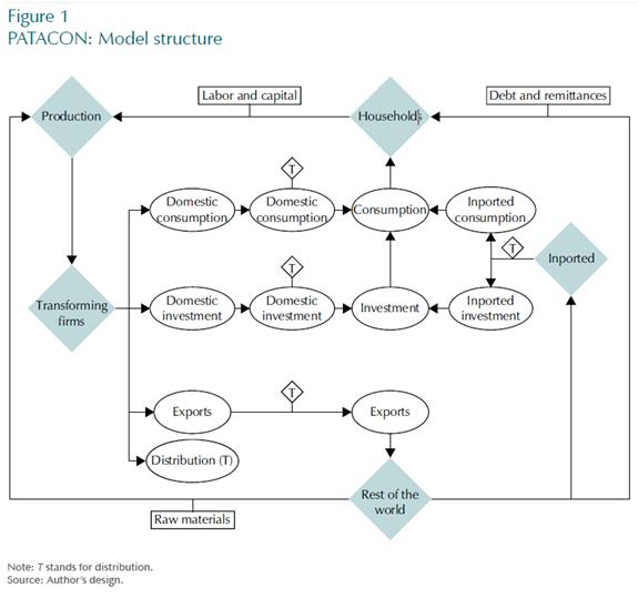
Similarly, imported goods are combined with distribution services by firms with some market power. Thus, the final price of imported goods is determined by both the foreign price and the cost of distribution in the domestic market. The latter implies an incomplete pass- through of the exchange rate to consumer prices. Parra (2010) and González et al. (2010) show evidence for this hypothesis. In general, the distribution allows for consumer and investment goods, both domestic and imported, to be purchased by households and exports to be sold abroad. Explicitly including the distribution services is one difference between PATACON and DSGE models calculated by Christiano et al. (2005), Smets and Wouters (2007) and Adolfson, Laséen, Lindé and Villani (2008).

Growth in the model is driven by population and trend productivity per worker, per hour worked. The economy is populated by a continuum of households. The total population of size grows at an exogenous rate . That is, 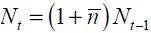Technological progress , is exogenous and follows the process 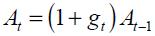where is a stationary variable and is described by 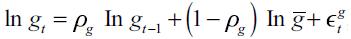, where is the steady state growth rate of the technological progress, , and .

To keep things simple, both the rate of labor force participation and the rate of unemployment are also exogenous in this economy. The number of people working during each period is , where is the unemployment rate from the economically active population and is the gross rate of participation from the total population. Both concepts correspond to series reported by the Colombian Department of National Statistics (DANE)². The model is solved for the stationary variables; and consequently, we express all variables in model units, effectively adjusting them for the two sources of growth, population and Harrod neutral technological progress and for convenience, also by total average number of hours in a quarter .

III. Households

There is a continuum of households indexed by j. These households solve three problems simultaneously: the first is maximizing utility subject to a budget constraint; the second is choosing the consumption bundle composition, between domestic and imported goods; and finally, since the households offer differentiated labor in a monopolistically competitive labor market, making their choice for the nominal wage.

A. Utility maximization

Household j seeks to maximize the discounted sum of its utility subject to a budget constraint. Its instantaneous utility function describes its preferences over consumption and leisure at any moment in time , where the consumption bundle and is the level of leisure. We assume that each household has a fixed allocation of time so that its leisure, relative to the total time, is given by , where is the fraction of hours spent working during the quarter.

The instantaneous utility function is the following:
,
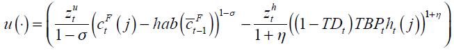where represents the intertemporal elasticity of substitution, is the habit consumption parameter, is last period final consumption, and is the inverse of Frisch 's elasticity. In addition, there are exogenous shocks to the marginal utility of consumption, , and to the marginal disutility of labor, .

It can be assumed that these exogenous shocks follow autoregressive processes.

The household owns the production factors, hours to work and physical capital . From the use of these production factors each household earns a real hourly wage rate, , and a real rental rate of capital, . Additionally, households receive real profits, , from firms and remittances, , from abroad. These remittances are exogenous in foreign currency and follow an autoregressive process.

The household buys Arrow-Debreu securities which are state contingent securities that insure the household against idiosyncratic shocks. As we shall see, wages are allowed to differ across households; however, with these securities, consumption plans of different households are identical. Since households are insured against idiosyncratic shocks, and have the same preferences; then it must be the case that all individual decisions are identical, except for the wage and fraction of hours worked. This enables us to drop the j subscript in the other variables.

As for the expenditures, the household buys the consumption bundle, at a price , and invests in capital stock by buying new investment goods, , at a price . Since investing is costly, we assume that the household covers the investment cost. This cost is proportional to changes in the investment rate, as in Christiano, Eichenbaum and Evans (2005) and it is described through the following equation:

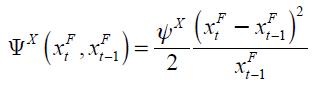
where is the adjustment cost parameter.

The household also chooses how intensively to work the capital. The rate of capital utilization is represented by . Through this decision the household will affect both the rent of capital and its depreciation rate. See Christiano et al. (2005). Additionally, the household has to cover the debt services in domestic and foreign currency. Net domestic assets, , earn nominal interest , and net foreign assets, , in nominal foreign currency terms, pay an interest rate . We denote the nominal exchange rate a , and the external consumption bundle price as .

We can aggregate across the households and express the aggregate budget constraint as:

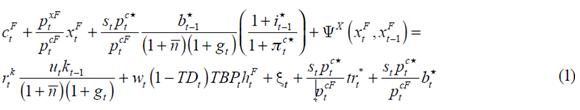
where 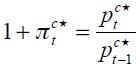is the external consumption bundle inflation in foreign currency that follows an exogenous process.

A second constraint faced by the economy is the capital accumulation equation, defined as:

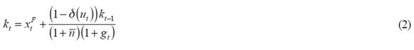
where is the endogenous depreciation rate, which is a function of the capital utilization:

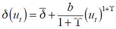
With as a parameter that affects the steady state rate of depreciation, a scale parameter, and a parameter that affects the dynamics of the capital depreciation rate.

Aggregating across households, the first-order conditions for this problem are:

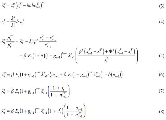
where 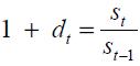denotes the nominal devaluation rate, is the subjective discount factor, and must be small enough to ensure that there will always be net discounting of the future. In particular, for given values of , and , , is constrained by .

Note that Equation (4) describes the trade-off in adjusting the degree of capacity utilization; Equations (5) and (6) describe the investment and capital stock decisions respectively, which are often used as the basis for partial equilibrium estimations of investment; Equations (3) and (7) jointly produce the standard Euler equation for intertemporal consumption. Finally, by combining Equations (7) and (8) we obtain the uncovered interest rate parity.

B. Domestic and imported consumption choice

In a separate hypothetical second stage, households choose consumption of domestically produced goods and imported goods by minimizing costs. The aggregate consumption bundle includes domestically produced goods, , and imported goods adapted for local consumption, . These are aggregated in utility as:

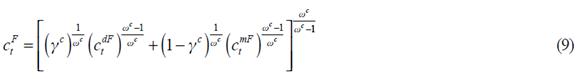
where is the elasticity of substitution between domestic consumption and imported consumption. controls the participation of domestic consumption on total consumption. The first-order conditions for the minimization problem are:

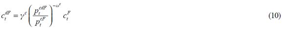
and:

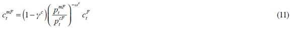
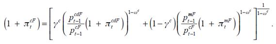
where is the price of domestically produced consumption and is the price of imported goods. By substituting Equations (10) and (11) into the consumption bundle we obtain the consumer price inflation:

C. Wage setting problem

The households offer differentiated labor in a monopolistically competitive labor market. But wages are rigid in nominal terms; it can therefore be assumed that each household must wait for a stochastic signal before adjusting the nominal wage rate. As in Erceg, Henderson and Levin (2000), households are hired by an intermediary firm which operates in perfect competition. This firm combines the work effort of households and supplies a joint labor input, . The demand for labor of household j is 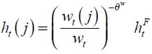, and the wage index is 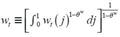, where represents the elasticity of substitution among differentiated labor from households.

Given the demand for its differentiated labor, the household optimally sets its wage when it receives a random signal which arrives every quarter with probability , this probability is independent from its own history and from other shocks in the model. The optimal wage, , is chosen so as to maximize the household's expected utility subject to the budget constraint and the consequent probability that it would not be able to reset its wage in the future. Notice that all households able to choose optimally will choose the same wage because the market for assets allows them to eliminate the idiosyncratic risk associated with not being able to adjust optimally in the future. We can therefore omit subscript j from the optimal wage. If the signal is not received, the wage is adjusted according to a rule. This rule implies that nominal wages increase in line with previous period inflation, .

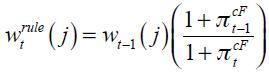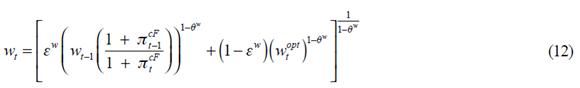
Additionally, it can be shown that aggregated real wage follows:

IV. Firms

The production structure of our model differs from the production structure found in other DSGE models. There are several reasons why we build a more complex production sector. First, we found that distribution of goods is an important component of the total cost of the final good (see Parra, 2010). Second, final goods are produced using both imported goods and domestically produced goods. Similarly, imported goods have to be distributed, and the distribution costs are not negligible.

The complete production process comprises four stages. First, a set of firms produces a domestic generic good (gross output). These firms combine domestic factors, such as labor and capital, with imported raw materials. In the second stage, the generic good is transformed into four different intermediate goods: domestic consumption goods, domestic investment goods, export goods, and distribution services. We call firms involved in this stage ¨transforming firms¨. These firms do not produce any value added. However, having this transforming stage in the model allows us to create a set of relative prices that is useful in the calibration process. In the third stage, a final producer combines the distribution services with intermediate goods to produce either a domestic consumption good, a domestic investment good, or export or import goods.

Finally, we have the producers of investment goods who combine the final domestic investment good with the imported investment good, and produce an aggregate investment good.

A. Gross output producers

There is a continuum of firms indexed by , wherein each firm produces a differentiated product, , sold at a price . These firms find themselves in a state of monopolistic competition and in each period have a constant probability of adjusting their price optimally. Therefore, they must solve two problems: first, they decide on their factors' demand for production, and then, they choose the output price upon receiving a stochastic signal that allows them to change the price.

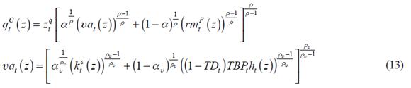
The production function is defined as:

where is the demand for capital³ from firm is the demand for labor in hours, is the demand for imported raw materials and is an aggregate temporary technology shock that follows an exogenous process. The price of raw materials, , depends on the nominal exchange rate through the price of imported raw materials at the dock, . This comes from the fact that purchasing power parity holds: that is, 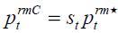, where is the external price of raw materials which we also assume to be exogenous. The difference between the price of raw materials at the dock and the final price of raw materials comes from the existence of nominal price rigidity.

Notice that the production function in Equation (13) implies different degrees of substitutability between value added and raw materials, and between capital and labor. This feature allows us to control the degree of substitutability between domestic and imported factors, see Bruno and Sachs (1985, p. 64). There exist elasticities of substitution between and and between and are and . The participation of in the value added is controlled by and the participation of in the production is controlled .

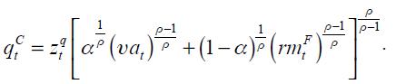
From the minimization problem, these firms determine their factor's demand:

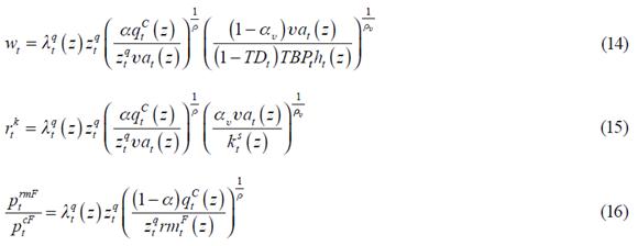
where the real marginal cost, , is derived as:

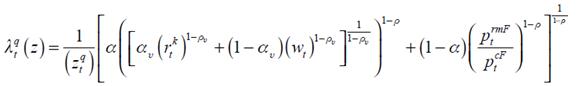
Note that is the same for every firm , because it depends on the aggregate wage rate, , the aggregate rent of capital, , the relative price of raw materials , as well as on the aggregate temporary technology shock, which is also common to all firms.

Each firm , as a producer of the differentiated intermediate good, faces a downward sloping demand curve of the form:
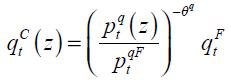, where 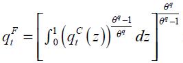is the gross output demand, is the aggregate price and is the elasticity of substitution among the firms.

The problem of setting prices is motivated by assuming that in each period firms face a constant probability of receiving a signal which tells them that they can adjust their price optimally. As in Calvo (1983), the representative firm will choose a price, , so that its expected stream of profits will be at its highest, given the constraint that it will only be allowed to change its price optimally on receipt of a random signal. The other firms set their price according to the following backward looking indexation rule: , where is the central bank's inflation target, is the weight assigned to past inflation as opposed to this target.

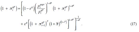
Given Calvo's pricing arrangement at each moment, the producer's inflation is given by⁴:

Finally, integrating across firms we obtain the output equilibrium condition: 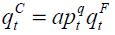where is the price distortion that appears from the fact that there are two fractions of firms adjusting at different prices (see Yun, 1996), is the aggregate demand for the raw good that must satisfy:

and is the total supply from all goods, defined as:

B. Transforming Firms

At a following stage, the generic raw base product is transformed into four different types of intermediate goods: domestic consumption goods, , domestic investment goods, , exports, , and distribution services, . An example of domestically produced consumption would be services. Construction is an example of a domestically produced investment good. In Colombia, oil, coal, nickel, coffee and industrial products are typical examples of export goods. And examples of domestically produced distribution services would basically include transport and commerce. These transforming firms take one input and produce four types of output using the following equation:

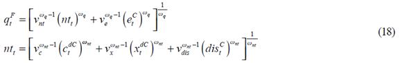
which represents the minimum quantity of real resources (in terms of the final good of the economy) that are needed to produce these many outputs, as in the Edwards and Végh (1997) model of banking production. In Equation (18), governs the elasticity of substitution between domestic uses of output and exports, and governs the elasticity of substitution among domestic uses of output. The parameters , , , , define the shares.

The functional form in Equation (18) assumes that substitution between export production and any other domestic use of output is not necessarily the same. In Colombia, nearly one half of export production is concentrated in four commodities which are often called "traditional exports". These goods (oil, coal, nickel and coffee) cannot easily be transformed for domestic use. That is why we should allow for a different elasticity to capture the special rigidity that emerges in the transforming that takes place between domestic production and traditional exports.

The first order conditions are given by the following supply functions:

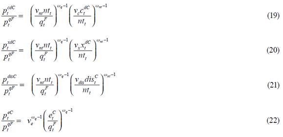
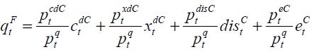
C. Final good producers

In every economy there is a sector which takes finished manufactured goods and brings them to the consumer. This sector combines retailing, marketing and transport. The role of this sector is becoming increasingly important as goods acquire the essential characteristic of services, which is to be designed for each consumer. The economics of this sector have a very important effect on final consumer prices, which is often referred to as distributor's margins. For example, they play a role in shaping the pass-through of exchange rate changes into the economy (see Campa and Goldberg, 2008). In this section, we describe how the output of that sector is used to transform the raw outputs of other sectors so that they are ready for final uses.

It is also described how the distribution sector transforms the intermediate goods into goods ready for final use. In what follows, is a dummy variable which could refer to domestic consumption, , domestic investment, , exports, , or imports . The superscript j represents , , or .

There is a continuum of firms, indexed by , which produces in monopolistic competition. These firms buy the intermediate good at a price , and combine it with the distribution sector's output, , to transform this intermediate good into a good ready for final use. As above, we assume a price setting structure, as in Calvo (1983), for the production of this final good and also in the production of the distribution services.

The production function for the final good is represented by:

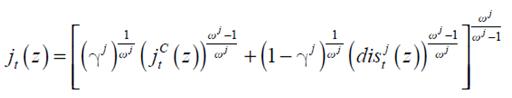
here represents the elasticity of substitution between distribution services output and other raw goods. is a participation coefficient. The demand for factors is:

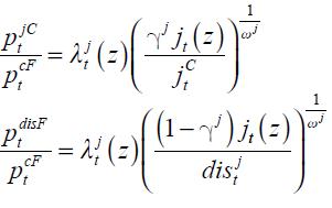
where is the marginal cost associated with producing good .

The market equilibrium condition for the good is, 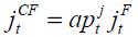where , is the price distortion, is the total supply from all firms in each sector and is the total demand for each sector output.

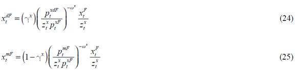
In the model, Equation (10) is the demand for final domestic consumption , Equation (24) is the demand for final domestic investment , Equation (5.1) is the demand for final exports and Equations (11) and (25) are the demands for imports. Finally, note that the price of the imports depends directly on the exchange rate since the purchasing power parity condition holds at the dock, that is, where, is the external price of imports that follows an exogenous process.

D. Investment producers

As we have seen, investment goods can be produced abroad and domestically. Both are important in explaining Colombian growth and fluctuations. An example of the former would be machinery, an example of the latter would be infrastructure. These two types of capital are aggregated to produce combined investment. This enables us to work with an aggregate capital stock in production. The technology for combining the two types of capital is described by:

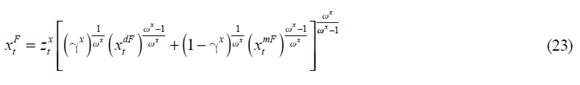
where is final investment, is the input of domestically produced investment, is the input of imported and distributed investment, is the elasticity of substitution between domestically and imported investment, defines the share of domestic investment into total investment, and is an investment efficiency shock. The expressions for the investment demands are:

V. Foreign variables

It is assumed that exports are demanded according to the following function:

where is the external demand that follows the autoregressive process, is the foreign currency price of Colombian exports and is defined as, .

Following Schmitt-Grohé and Uribe (2003) we impose a further condition to ensure that external debt converges into a predetermined ratio with GDP. Let us assume that the external sector offers resources at a rate, , which depends on the deviation of debt from this target ratio. In that case, we define the rate of interest as:

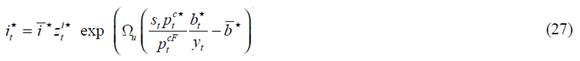
where is the nominal risk-free international interest rate, is the external debt to gross domestic product ratio, is its target value, is a parameter that affects the model dynamics, and is a risk-premium shock which follows an exogenous process.

VI. Monetary policy

Monetary policy in the model follows the simple rule:

where is the smoothing coefficient, is the steady state value for the nominal interest rate, determines the response to deviations in the inflation from its target, is the level of output if prices were flexible, and is the response to deviations of GDP from its flexible prices´ value. Deviations from the observed nominal interest rate and the nominal interest rate dictated by this rule are defined by the exogenous process .

VII. Conclusions and further research

In this document we have described the structure of PATACON, a DSGE model for the Colombian economy. PATACON was designed to be useful for analyzing Colombian macroeconomic data and to help guide monetary policy discussion. The data used in the model was constructed by Mahadeva and Parra (2008), who have described the construction of a data set that is used to calibrate the model. Bonaldi et al. (2011) propose an algorithm for calibrating the steady state ratios and relative prices according to the data. Bonaldi et al. (2011a) and Bonaldi et al. (2011b) describe the estimation of the model and present impulse response analysis, and, finally, González et al. (2011) describe how the model can be used for taking account of real world features of the data.

However, in its design we have ignored three characteristics of the Colombian economy that may be important. The first omission in PATACON is that it does not incorporate frictions in the labor market, and consequently, it cannot explain the dynamics of employment and unemployment over the business cycle. An initial attempt to incorporate these features in a DSGE model for the Colombian economy can be found in González, Ocampo, Rodríguez and Rodríguez (2011). The second omission is not having made the introduction of the financial sector so as to better understand its role in the economic business cycle. Some initial work has also been done on this aspect. See, for example, López and Rodríguez (2008); López, Prada and Rodríguez (2009); López and Prada (2010) or Bustamante (2011). And finally, the third omission is the lack of an explicit modelling of the government sector.

Comments

¹ Imports plus exports are about 45% of Colombia's GDP.

² Departamento Administrativo Nacional de Estadística, Colombia.

³ Aggregating the demand for capital across all firms equals the total supply of capital given by

² Since all firms are identical and then That is, all adjusting firms choose the same price.

REFERENCES

1. Adolfson, M.; Laséen, S.; Lindé, J.;Villani, M. "Evaluating an Estimated New Keynesian Small Open Economy Model", Journal of Economic Dynamics and Control, vol. 32, num. 8, pp.2690-2721, 2008.         [ Links ]

2. Bonaldi, P.; González, A.; Prada, J. D.; Rodríguez, D.; Rojas, l. E. "Método numérico para la calibración de un modelo DSGE", Revista Desarrollo y Sociedad, núm. 67, pp. 119-156 2011.         [ Links ]

3. Bonaldi, P.; González, A.; Rodríguez, D. "Estimating PATACON", Discussion Paper, Banco de la República of Colombia, 2011a.         [ Links ]

4. Bonaldi, P.; González, A.; Rodríguez, D. "Importancia de las rigideces nominales y reales en Colombia: un enfoque de equilibrio general dinámico y estocástico," Ensayos sobre Política Económica, núm. 66, 2011b.         [ Links ]

5. Bruno, M.; Sachs, J. Economics of Worldwide Stagflation. Harvard University Press, 1985.         [ Links ]

6. Burriel, P. F. V. J.; Rubio-Ramirez, J. F. "MEDEA: A DSGE Model for the Spanish Economy", PIER Working Paper, num. 09-017, 2009.         [ Links ]

7. Bustamante, C. "Política monetaria contracíclica y encaje bancario", Borradores de Economía, num. 646, Banco de la República of Colombia, 2011.         [ Links ]

8. Calvo, G. A. "Staggered Prices in a Utility-Maximizing Framework", Journal of Monetary Economics, vol. 12, num. 3, pp. 383-398, 1983.         [ Links ]

9. Campa, J. M.; Goldberg, L. S. "Pass-Through of Exchange Rates to Consumption Prices: What Has Changed and Why?", in International Financial Issues in the Pacific Rim: Global Imbalances, Financial Liberalization, and Exchange Rate Policy (NBER-EASE Volume 17), NBER Chapters, pp. 139-176. National Bureau of Economic Research, Inc., 2008.         [ Links ]

10. Christiano, L. J.; Eichenbaum, M.; Evans, C. L. "Nominal Rigidities and the Dynamic Effects of a Shock to Monetary Policy", Journal of Political Economy, vol. 113, num. 1, pp. 1-45, 2005.         [ Links ]

11. Christiano, L. J.; Trabandt, M.; Walentin, K. "Introducing Financial Frictions and Unemployment into a Small Open Economy Model", Working Paper Series, num. 214, Sveriges Riksbank (Central Bank of Sweden), 2007.         [ Links ]

12. Edwards, S.; Végh, C. "Banks and Macroeconomic Disturbances Under Predetermined Exchange Rate", Journal of Monetary Economics, num. 40, pp. 239-278, 1997.         [ Links ]

13. Edwards, S.; Végh, C. "Banks and Macroeconomic Disturbances Under Predetermined Exchange Rate", Journal of Monetary Economics, num. 40, pp. 239-278, 1997.         [ Links ]

14. González, A.: Mahadeva, L.; Rodríguez, D.; Rojas, L. E. "Monetary Policy Forecasting in a DSGE Model with Data that is Uncertain, Unbalanced and About the Future", Ensayos sobre Política Económica, num. 66, 2011.         [ Links ]

15. González, A.; Ocampo, S.; Rodríguez, D.; Rodríguez, N. "Asimetrías del empleo y el producto, una aproximación de equilibrio general", Borradores de Economía, num. 663, Banco de la República of Colombia, 2011.         [ Links ]

16. González, A.; Rincón, H.; Rodríguez, N. "La transmisión de los choques a la tasa de cambio sobre la inflación de los bienes importados en presencia de asimetrías", in M. Jalil and L. Mahadeva (Eds.), Mecanismos de transmisión de la política monetaria en Colombia (chap. 10), Bogotá, Banco de la República y Universidad Externado de Colombia, 2010.         [ Links ]

17. Hofstetter, M. "Sticky Prices and Moderate Inflation", Economic Modelling, vol. 27, num. 2, pp. 535-546, 2010.         [ Links ]

18. Iregui, A. M.; Melo, L. A.; Ramírez, M. T. "Are wages Rigid in Colombia?: Empirical Evidence Based On a Sample of Wages at the Firm Level", Borradores de Economía, num. 571, Banco de la República of Colombia, 2009.         [ Links ]

19. Julio, J. M. "Heterogeneidad observada y no observada en la formación de los precios del IPC colombiano", Ensayos sobre Política Económica, num. 63, pp. 66-99, 2010.         [ Links ]

20. Julio, J. M.; Zárate, 20. H. M.; Hernández, M. D. "The Stickiness of Colombian Consumer Prices", Ensayos sobre Política Económica, num. 63, pp. 100-153, 2010.         [ Links ]

21. López, M. R.; Prada, J. D. "Optimal Monetary Policy and Asset Prices: The Case of Colombia", Ensayos sobre Política Económica, vol. 28, num. 61, 2010.         [ Links ]

22. López, M. R.; Prada, J. D.; Rodríguez, N. "Evidence for a Financial Accelerator in a Small Open Economy, and Implications for Monetary Policy", Ensayos sobre Política Económica, vol. 27, num. 60, 2009.         [ Links ]

23. López, M. R.; Rodríguez, N. "Financial Accelerator Mechanism: Evidence for Colombia", Borradores de Economía, num. 481, Banco de la República of Colombia, 2008.         [ Links ]

24. Mahadeva, L.; Gómez, J. G. "Los factores externos que afectan la política monetaria colombiana", in M. Jalil and L. Mahadeva (Eds.), Mecanismos de transmisión de la política monetaria en Colombia (chap. 1), Bogotá, Banco de la República y Universidad Externado de Colombia, 2010.         [ Links ]

25. Mahadeva, L.; Parra, J. C. "Testing a DSGE Model and Its Partner Database", Borradores de Economía, num. 478, Banco de la República of Colombia, 2008.         [ Links ]

26. Misas, M.; López, E.; Parra, J. C. "La formación de precios en las empresas colombianas: evidencia a partir de una encuesta directa", Borradores de Economía, num. 569, Banco de la República of Colombia, 2009.         [ Links ]

27. Parra, J. "La sensibilidad de los precios del consumidor a la tasa de cambio en Colombia: una medición de largo plazo", in M. Jalil and L. Mahadeva (Eds.), Mecanismos de transmisión de la política monetaria en Colombia (chap. 9), Bogotá, Banco de la República y Universidad Externado of Colombia, 2010.         [ Links ]

28. Schmitt-Grohé, S.; Uribe, M. "Closing Small Open Economy Models", Journal of International Economics, vol. 61, num. 1, pp. 163-185, 2003.         [ Links ]

29. Smets, F.; Wouters, R. "Shocks and Frictions in US Business Cycles: A Bayesian DSGE Approach", American Economic Review, vol. 97, num. 3, pp. 586-606, 2007.         [ Links ]

30. Yun, T. "Nominal Price Rigidity, Money Supply Endogeneity, and Business Cycles", Journal of Monetary Economics, vol. 37, num. 8, pp. 345-370, 1996.         [ Links ]