


Services on Demand
Journal
Article
 English (pdf)
 Article in xml format
 Article references
 Send this article by e-mail
Indicators
-
 Cited by SciELO
 -
 Access statistics
Related links
-
 Cited by Google
 -
 Similars in
SciELO
Similars in
SciELO -
 Similars in Google
Share

 Permalink
Ensayos sobre POLÍTICA ECONÓMICA
Print version ISSN 0120-4483
Ens. polit. econ. vol.32 no.spe73 Bogotá Jan. 2014
Uncertainty in the Money Supply Mechanism and Interbank Markets in Colombia*
Incertidumbre en el mecanismo de oferta monetaria y mercados interbancarios en Colombia
Camilo Gonzáleza, Luisa Silvaa, Carmiña Vargasa, and Andrés M. Velascoa
* This work represents the sole opinions of the authors and not those of the Board members of the Banco de la República de Colombia.
a Banco de la República, Bogotá, Colombia
E-mail addresses: cgonzasa@banrep.gov.co (C. González); lsilvaes@banrep.gov.co (L. Silva); cvargari@banrep.gov.co (C. Vargas); avelasma@banrep.gov.co (A.M. Velasco).
History of the article:Received June 28, 2013 Accepted December 17, 2013
ABSTRACT
We set a dynamic stochastic model for the interbank daily market for funds in Colombia. The framework features exogenous reserve requirements and requirement period, competitive trading among heterogeneous commercial banks, daily open market operations held by the Central Bank (auctions and window facilities), and idiosyncratic demand shocks and uncertainty in the daily auction. Analytical derivations of their decision making process show that banks involvement in the interbank market and open market operations depend on their individual requirement constraint and daily liquid assets. Our results do not show a linkage between the uncertainty in the money supply mechanism and activity in the interbank market. Equilibrium interest rate for the interbank market is derived, and is shown that it is distorted by uncertainty at the daily auction held by the monetary authority. Using data for Colombia, we test the main results of the model and corroborate the Martingale hypothesis for the interbank interest rate.
Keywords: Interbank market, Overnight rates, Reserve demand.
JEL Classification: E44, E52, G21.
RESUMEN
En este documento se plantea un modelo dinámico estocástico para el mercado interbancario diario en Colombia. La configuración del modelo incorpora bancos comerciales heterogéneos que interactúan en un entorno competitivo, operaciones de mercado abierto (OMA) diarias realizadas por el Banco Central (subastas y ventanillas), incertidumbre en la obtención de recursos en la subasta diaria, choques de demanda idiosincráticos y requerimientos de reserva definidos exógenamente. Las derivaciones analíticas acerca del proceso de toma de decisiones de los bancos muestran que la participación de cada entidad en el mercado interbancario y en las OMA dependen de su requerimiento de reserva y del nivel de sus activos líquidos diarios. En los resultados obtenidos no se evidencia algún vínculo entre la incertidumbre en el mecanismo de oferta monetaria y la actividad en el mercado interbancario. En particular, se encuentra la tasa de interés de equilibrio para el mercado, y se muestra que está distorsionada por la incertidumbre en la obtención de fondos en la subasta diaria. Finalmente, utilizando datos para Colombia, se prueban los principales resultados del modelo y se corrobora la hipótesis de Martingala para la tasa de interés interbancaria.
Palabras clave: Mercado interbancario, Tasa de interés interbancaria, Choques de liquidez, Demanda por reservas.
Clasificación JEL: E44, E52, G21.
1. Introduction
The correct functioning of interbank markets is important among other reasons because banks can redistribute cash reserves among its participants, and because interest rates reached in these markets provide a benchmark for other sectors of the economy.
Regarding liquidity management, banks can smooth liquidity shocks by borrowing or lending in the interbank market rather than prematurely cancel more profitable longer-term projects. Thus, due to these markets, it is possible to avoid inefficient hoarding of reserves as a precaution against unexpected liquidity shocks. In addition, interbank markets play a key role in the transmission mechanism of monetary policy through the credit channel under the inflation targeting regime.
We have two main motivations in writing this paper. First we aim to understand how interbank markets work, and second, how Central Banks mechanism to conduct monetary policy affects outcomes (interest rates and loans) in those markets. Even though we focus our attention in the Colombian case, the analytical tools we develop here can be used to study a wide range of interbank markets from different economies since they have some common features.
This paper is composed by four sections, including this introduction that in what follows elaborates in our two main motivations. In section two we set a model for the interbank market in Colombia. The third section presents the data analysis for the case of Colombia in which we validate our analytical findings, and finally the fourth section concludes with some final remarks.
1.1. How Do Interbank Markets Work?
It is important to understand the monetary policy framework in which interbank activity takes place. As many other countries, Colombia established a floating exchange rate regime and started the process of converging towards an inflation targeting regime in the late nineteen nineties. During this process, monetary aggregates were replaced by the interest rate as the instrument used by the Central Bank.
The starting point is the announcement of an inflation target for a future period, usually one to two years ahead, which seeks to anchor inflation expectations of private agents in the economy. In this sense, theoretically, when there are shocks to the economy, the Central Bank changes the policy interest rate to bring inflation back into line with the target, and to maintain the economy around its long-term trend.
It is expected that when the Central Bank changes its policy interest rate, this immediately affects the interbank interest rate resulting in changes in short and long term interest rates in the markets. Therefore, the alignment between the policy interest rate and the interest rate in the interbank market is a necessary condition for the success of the monetary policy. It ensures the correct operation of the monetary transmission channels and, ultimately, the fulfillment of the inflation target as well as an output gap close to zero.
In Colombia, monetary policy works through auctions and window facilities. Instead of controlling the interest rate directly, the Central Bank supplies resources in a daily basis through auctions with amounts announced a day before; and administers deposit and lending facilities to allow financial institutions to let or get overnight resources at or from the Central Bank, respectively. The aim of the monetary authority is to supply just enough resources to keep the auction rate in line with the policy rate every day. The aim of commercial banks and other interbank market participants is understood to be to maximize profits subject to liquid asset holdings, obligations to other banks and the requirement constraint the Central Bank sets to diminish deposit default risks.
Trading day activity in the Colombian monetary market is not too simple. The complexity arises due to a variety of possible operations and counterparts. As explained by Cardozo, et al. (2011), there are collateralized and uncollateralized trading that takes place in electronic negotiation systems or in OTC (Over-the-counter) markets. Furthermore, a wide range of institutions are able to trade in these markets (banks, bank-like institutions, stockbrokers, among others) and the Central Bank holds open market operations (OMO) at certain and known hours in a day.
Trading days start at 7 a.m., when Colombia's large-value payment system (CUD, in Spanish) and SEBRA (electronic services provided by the Banco de la República) open. At 8 a.m., institutions start trading in electronic negotiation systems like SEN and MEC1. Operations in SEN go until 1 p.m., while those in MEC go until 5 p.m. Although banks can trade and negotiate until 5 p.m., most of the activity in the interbank market occurs before 1 p.m.
Central Bank holds two main OMOs: a) auctions for funds by REPOS (1 p.m.),2 and b) lending and deposit facilities (4 p.m.). The amounts auctioned are bounded by the Central Bank. Commercial banks and bank-like institutions compete under a Dutch auction system. With the window facilities, the Central Bank lends or borrows funds without setting a maximum amount, but charging or paying interest rates different from the official policy interest rate.
In section 2, we present a model that tries to capture stylized facts shown in Figures 1 and 2:
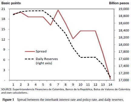
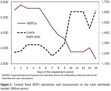
Figure 1 shows average data for each of the 14 days in the requirement period in Colombia. Spread accounts for the difference between the aggregate (collateralized and non-collateralized operations) interbank interest rate and the policy rate (left axis). Daily reserves shows average holdings of liquidity by institutions, to contribute to their reserve requirement constraint (right axis).
We analyze the period January 2012 to April 2013. It looks as if banks follow a reserve strategy in which they contribute to their reserve requirement with big amounts at the beginning of the reserve period. With respect to the spread between the interbank interest rate and the policy rate, it is also decreasing. In the first days, the spread is around 20 basis points, but throughout the two weeks it is reduced to a level close to zero in the last day. Consistent with their desire to quickly contribute to their reserve requirement, commercial banks are willing to pay higher interest rates in the interbank market at the beginning of the reserve period.
Figure 2 show aggregate demand at the daily auction (left axis), and average supply of resources in the interbank market (right axis). Consistent with the reserve strategy shown in Figure 1, commercial banks demand more resources in the auctions held in the first days of the reserve period, and offer relatively little liquidity in the interbank market.3 This situation is reversed towards the end of the two-weeks period.
It is worth noticing that demand for funds in the 13th day does not follow the trend described above. We infer this behavior responds to precautionary decisions by banks: since there is a chance of suffering negative demand shocks the last day of the maintenance period (when their constraint binds), institutions reduce their lending amounts and demand more funds both at the auction and in the interbank market.
Section 3 presents empirical analysis of model in section 2. The model we set explains nearly 80% of variance of contribution to the reserve requirement, nearly 95% of variance of the interbank interest rates and nearly 28% of variance of daily activity in the interbank market. We consider this a satisfactory result given that this is a very stylized model of an interbank market.
1.2. How the Monetary Policy Mechanism Affects Interbank Markets?
In theory, the inflation-targeting-regime policy tool is the interest rate, particularly, the policy rate that the monetary authority fixes at the desired level to offset shocks to the economy, and take it to its steady state. An alternative to this mechanism involves two rates separated by a spread to provide and receive liquidity to and from markets.
In Colombia, as in many other economies (we show below), policy mechanism acts through REPO auctions and lending and deposit facilities to implement monetary policy. Cardozo et al. (2011) argue in favour of two advantages for having this system compared to a system with one or two explicit interest rates through which all liquidity is managed:
-
It encourages the deepening of the interbank market, which is useful to extract signals and evaluate solvency and risks taking by its participants.
-
It reduces the possibility of excessive leverage by the financial system, which may be used to speculate on the foreign exchange or securities markets.
This paper focuses on providing an analytical tool to evaluate the first reason. We do not assess the second one. In order to understand how the interbank market works in Colombia, we construct a framework that allows us to assess the relationship between the mechanism through which the Central Bank provides liquidity and the overall interbank market.
The Colombian mechanism to implement the monetary policy shares most of the features with other countries operating under an (implicit or explicit) inflation targeting regime. In fact, a survey of 16 central banks (Australia, Brazil, Canada, Chile, Colombia, United States, Europe, Japan, Mexico, Norway, New Zealand, Peru, England, South Africa, Sweden, and Turkey) shows the following:
- All of them have some overnight interest rate as the operative instrument (either, the interest rate for non-collateralized credit or the interest rate for collateralized credit).
- 15 out of the 16 banks use REPO at auctions, but they differ in frequency and maturity.
- All these central banks administer lending and deposit facilities.
- Reserve requirement is less common, only 9 out of 16. Inefficiency and heterogenous treatment among competitors are examples of reasons claimed for not using it.
- Furthermore, central banks regulate the liquidity in a more permanent way by buying or selling securities and international reserves. In the first case, the securities can be issued by governments or, in some cases, by central banks themselves.
Given that this money supply mechanism is widely used among inflation targeters, we think it is important to ask how the policy structure affects the interbank market. Our analytical results in section 2 allow us to conclude that activity in the interbank market is not affected by uncertainty in the daily auction, however it distorts the interbank interest rate. Our results show that when the monetary authority commits to providing with certainty all the liquidity demanded by all institutions at the policy rate, the interbank interest rate is equal to the policy rate.
2. Model
We describe a model for the interbank daily market for overnight funds in Colombia. The structure of the model follows some features of the problem-setting, derivation and solution in Pérez and Rodriguez (2006).
We are not the first in building on the framework proposed by Pérez and Rodriguez (2006) (PR, 2006, from now on): Cardozo, et al. (2011) set a framework with the Colombian timing, but do not include sources of uncertainty, of which we have two. Perez and Rodriguez (2010) allow for an extra facility in which commercial banks clear their accounts between them and with the Central Bank. This facility is designed to be occasional and the banks have uncertainty over it. Kempa (2006) models common and idiosyncratic shocks, and Kempa (2007) includes expected innovations in the demand for resources faced by banks along with the demand shocks. Jurgilas (2006) introduces heterogenous banks, and the possibility for foreign funding for them. Moschitz (2004) models the supply side in detail from the perspective of the balance sheet of the Central Bank, setting an explicit objective function for it.
We modify the structure of the model in PR (2006) in four aspects: first, we allow for daily auctions instead of one in the entire requirement period; second, we alter the timing of the model to have the auction after interbank trading has taken place, at any given day, and not before; third, the banks in our model optimally decide over the amount of reserves they accumulate each day to contribute to their reserve requirement, which is a residual in PR (2006). In this paper we present one of four possible timings for this decision to be made: simultaneously with the auction demand decision.4 Fourth, along with the demand shock in PR (2006), banks in our model face a second source of uncertainty: there is a probability of not obtaining resources at the auction, which is a shortcut for modelling an auction mechanism. Finally, the reader should note that our framework does not take into account frictions that would alter the perfect competition assumption, nor other sources of heterogeneity among institutions (e.g., size), neither risk perception between market participants (or other information problems).
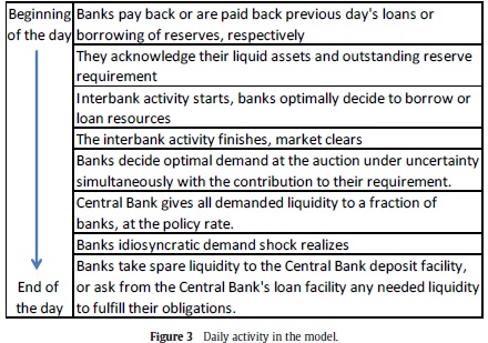
We model a single reserve period where interbank daily activity is characterized by the following timing: commercial banks start the day by paying back or being paid back for interbank and auction interactions in the previous day. At that point they find out their liquid assets and their outstanding reserve requirement. They trade in the interbank market to maximize their benefits with uncertainty about future supply (at the auction) and demand (at the en of the day) shocks. Once the interbank trading has finished and cleared, they decide optimally how much to demand in the daily auction. We proxy this OMO by assuming that only a fraction of banks obtains all the liquidity they have demanded, while the rest obtains no extra liquidity from the auction. At this time of day, simultaneously with the auction, we assume that banks in our model decide how much they will keep in reserve at the end of the day to contribute to their reserve requirement. After the auction, banks find out the size of their daily idiosyncratic demand shock, typically coming from their clients. They take any spare liquidity they have at the end of the trading day to the deposit facility at the Central Bank; or they get any needed liquidity from the lending facility also at the Central Bank. Figure 3 presents a summary of the described daily timing.
2.1. Set Up
Consider a continuum of heterogenous commercial banks of size one, indexed by j, that trade in a competitive fashion over daily reserves. There is a Central Bank that provides liquidity through auctions and windows every working-day, and that has established a requirement period of T calendar days. We set the model for a single requirement period, and assume periods of T days independent of each other to avoid an infinite horizon and the necessity for discount rates. The Central Bank sets each bank's requirement exogenously from the model. Banks hold reserves at the end of each day to complete the T-days-average heterogenous amount, Qj, required.
We follow PR (2006) in defining the deficiency, rj,t, as the amount of reserves the bank j is short from the total requirement of T · Qj, at time t. According to this, banks satisfy their reserve requirement when
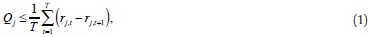
where each day during the requirement period, bank j starts with deficiency rj,t and decides on its next day's deficiency rj,t+1. Then rj,t - rj,t+1 is the reserve that the bank j leaves at the end of the day t to contribute to its requirement constraint.5 Note that in the last day of the requirement period T, the requirement constraint is binding, therefore banks set their next day's deficiency to zero (i.e. rj,T+1 = 0).
Daily reserves have both stochastic and deterministic components that will be defined shortly.
At the beginning of every trading day t ∈[1,T] , commercial banks meet at the interbank market and supply (bj,t > 0) or demand (bj,t < 0) net resources to maximize benefits, subject to their heterogenous asset holdings, αj,t, at the beginning of the day t. Banks clear the interbank market at the interest rate it.
Once the interbank trading activity has finished for the day, the Central Bank holds its daily auction to provide the financial system with liquidity. Banks decide about demand resources (dj,t) by maximizing its expected profits given an expected auction interest rate Et(iomo,t).6 We introduce supply uncertainty assuming each bank gets the resources it has previously decided to demand with probability p ∈ [0,1], but with probability 1 - p it leaves empty handed. Therefore for every day t, a fraction p of all institutions receive the liquidity they demanded.
In our model, the Central Bank starts transmitting the monetary policy stance by providing all the liquidity demanded in the daily auction at the policy interest rate ip. As information is common to all agents, we can expect commercial banks will generate expectations over the auction rate such that

Daily available reserves for bank j, before the auction in day t (mj,t), are defined as

where the indicator function I(p) takes the value of one when bank j has been drawn to get its demanded liquidity at the auction, with probability p, at time t; and zero otherwise, with probability 1 – p.
Note that equation (2) does not make explicit reference to payments of previous day's auction demand/supply or interbank activity. This is because mj,t is defined as a net flow: re-payments in the interbank market and to the Central Bank have taken place at the beginning of the day.
We have departed from model in PR (2006) by having a supply shock, but also by allowing banks to optimally decide how much of the available daily reserves they use to reduce its next day deficiency, rj,t+1. This decision is arbitrarily assumed to be taken simultaneously with the decision about dj,t at the daily auction.
After the daily auction, banks realize they have been hit by a demand shock for resources 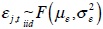 , typically coming from their clients. This shock is of the same nature as the one described by PR (2006) and assumed to be identically and independently distributed across time and banks.
Equation (3) summarizes daily reserves' sources (in the right-hand side) and uses (in the left-hand side):

where we define ej,t as residual reserves after supply and demand shocks, which do not contribute to reduce the deficiency. If ej,t> 0, the bank takes those resources to the deposit facility at the Central Bank, that yields id. If ej,t< 0, the bank demands those resources from the lending facility at the Central Bank, at the cost il, since banks are not allowed to go overdraft through the night and they have to honour their requirement constraint at time T.
Asset holdings by bank at the beginning of the next day are given by7

A solution for the model is the set of equilibrium interbank interest rates, {i*t}, for each day of the requirement period, t ∈[1,T] .
The equilibrium interest rates are determined by the clearing market condition:
We follow PR (2006) in solving the model by backward induction. We start by describing decisions at the last-day-of-the-reserve-period auction, to then move backwards to the beginning of that day, T. Then we continue describing decisions at T – 1, first at the auction followed by the interbank activity, and we finish showing recursiveness in the previous days of the reserve requirement period.
2.2. Payoffs and Solution at the Last Day of the Reserve Period
2.2.1. Bank's Problem at the Last Day Auction
At period T, commercial bank j faces the auction having traded for the last time in the interbank market in the current reserve period. It decides its demand for liquidity, dj,T, to maximize the expected value of its profits, with uncertainty about whether it will get the money demanded, with probability p, and about the demand shock, εj,T, that is only realized before the end of the day after the auction has taken place.
The bank knows that after the auction it will find itself in one of three situations: the bank might need resources to reduce its deficiency to zero, since the requirement constraint binds in period t. In this case it has to lend the amount needed from the Central Bank facility, at the interest rate il . The other two situations either leave the bank in perfect balance or with excess liquidity that the bank will deposit at the Central Bank. As discussed before, this yields id overnight.
Up to this time, the bank knows its assets (αj,T), outstanding deficiency (rj,T), policy and facility rates from the Central Bank (ip, id and il), and the distribution of supply and demand shocks (B(p) and F(με,σ2ε)). The bank knows that the requirement constraint is binding ( rj,T +1=0), then it maximizes its profits at the auction conditional to its involvement in the interbank market earlier in the day (bj,T). The bank solves

where
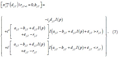
where, again, the indicator function I(·) takes the vale of one when the condition inside the parenthesis holds, and zero otherwise.
In the first line of (7), the bank pays the policy rate for its demand, dj,T, when realization of supply shock favours it. Subject to the realization of the demand shock εj,T, the bank either: a) saves money at the deposit facility when resources available are greater than the reduction to zero of outstanding deficiency, or b) asks for reserves at the Central Bank's facility when resources available fall short of outstanding deficiency. Note that with probability 1 – p the bank gets nothing at the auction. Then, expected profits previous to the last-day auction are given by
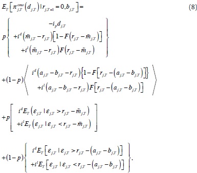
where we define  j,t = aj,t - bj,t + dj,t as reserves before the demand shock of bank j in the event that liquidity has been provided at the auction at time t ∈[1,T].
First order condition to the problem in (6) gives:
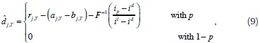
where we define reaction function with a hat over the variable, e.g.  . Then,
  j,T denotes the reaction function of bank j for demand of resources at the auction, conditional on shock distributions and predetermined bj,T.
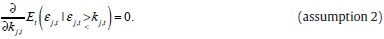
Note that in deriving (9) we follow PR (2006) in assuming that, for any kj,t conditioning the expected value of the demand shock, it holds that
Replacing (9) in (8), it is straight forward to see that marginal supply of resources in the interbank market earlier in the day affects the objective function before the auction as follows:
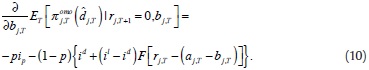
Marginal supply of liquidity in the interbank market reduces profits at the auction. Obtaining that marginal liquidity costs the policy rate with probability p, or, depending on the size of the demand shock a cost between the lending and the deposit rates from the Central Bank facilities with probability 1 - p. A positive demand shock reduces the probability of having to visit the lending facility of the Central Bank and reduces the cost. A negative demand shock increases the probability of having to visit the lending facility of the Central Bank and increases the cost.
2.2.2. Bank's Problem at the Last Day's Interbank Market
We continue solving the bank's problem at time T by backward induction. Now we focus in the beginning-of-the-day maximization problem. Bank j maximizes the day's profits by choosing its supply (or demand) in the interbank market, taking into account the reaction function in (9). The bank solves the beginning-of-the-day value function:
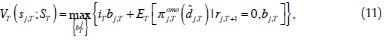
where the state of bank j at time T is defined by its reserve position  , and the aggregate state variable at time T is given by the interbank market rates up to T - 1, St = (i1,i2 ...iT-1).
The value function has two arguments: first, the bank decides how much to lend or borrow in the interbank market, and receives or pays the interbank interest rate, iT, respectively; and second, the expected value of bank's profits before the auction evaluated at its optimum.
Using (10), the first order condition of (11) is:

From (12), we solve for the reaction function of bank j for the liquidity supply (or demand) in the interbank market in the last day of the reserve period T:
Note that the reaction function of the liquidity supply (or demand) by bank j depends on the equilibrium interbank interest rate, iT; the state variables, αj,T and rj,T; exogenous rates ip, id and il, and shocks distributions.
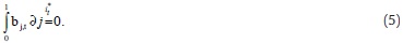
We use the clearing condition of the interbank market in (5) to obtain the last day's equilibrium interbank interest rate:

where we define aggregate variable Xt =  xj,t ∂j, for xj,t = (aj,t, bj,t, rj,t).
The equilibrium interbank interest rate is equal to the policy rate, ip, only if the probability of receiving the demanded resources at the auction is equal to one, i.e. p = 1. Otherwise, with p < 1, the mechanism for money supply causes a distortion that separates the equilibrium interbank interest rate from the policy rate. The spread between these two rates depends on the size of the expected demand shocks, and is bounded by the rates at the Central Bank's facilities.
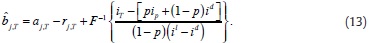
We replace equation (14) in (13) to obtain equilibrium supply of (or demand for) resources in the interbank market in the last day of the reserve period, by bank j:

Optimal activity of bank j in the interbank market in the last day of the reserve period depends positively on its assets net of its deficiency, and aggregate demand for resources (aggregate deficiency net of aggregate assets).
Note that the equilibrium supply of resources in the interbank market does not depend on the uncertainty of receiving resources at the auction. Therefore, we conclude that, at least under the framework presented for the last day of the requirement period, the money supply mechanism with auction and window facilities does not encourage the deepening of the interbank market.
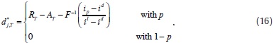
Replacing (15) in (9), we obtain equilibrium demand at the auction:
and aggregating over institutions that get liquidity at the auction, we obtain total supply by the Central Bank at time T:
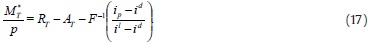
Equations (14) through (17) summarize the findings of the model for the last day of the requirement period, that are to be validated in section 3 of the paper. To continue with the backward induction it is useful to calculate how the value function in T changes with marginal changes in last period deficiency, rj,T. Then, replacing (16) in the value function in (11), we calculate:
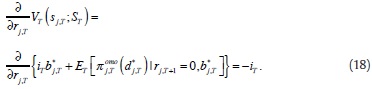
Marginal liquidity that was not used in T – 1 to reduce the deficiency with which the bank starts the last day of the reserve period, must be obtained in T either in the interbank market at the beginning of day T, or later under supply uncertainty in the last day's auction. Equation (18) shows that the opportunity cost of not marginally reducing the deficiency in T – 1 is the interbank interest rate, iT.
2.3. Payoffs and Solution at Time t = T – 1
2.3.1. Bank's Problem at the Auction in Day T – 1
We continue solving the model with backward induction for the auction in the-day-before-the-last, t = T – 1. At this time, the bank has found an equilibrium solution for endogenous variables in T, in terms of states, exogenous variables and parameters; and knows its assets and deficiency (aj,T–1, rj,T–1), Central Bank policy and facilities' interest rates and shocks distributions. At this time the requirement constraint is not yet binding, so the bank chooses over its demand at the auction, dj,T–1 , and next period deficiency, rj,T, to solve:

Objective function in (19) is composed by two arguments: first, it contains profits at the auction, and second, it contains next day value function evaluated at the equilibrium, but conditional on states which are determined in T – 1.8
We can write the first argument in (19) as:
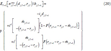
The first curly bracket in (20) shows the payoffs for the event in which the bank receives the liquidity demanded at the auction, with probability p: it pays the policy interest rate for liquidity demanded, and depending on states, decisions and the size and sign of the demand shock, the bank ends the day with spare liquidity (when εj,T –1 + j,T –1> rj,T –1 – rj,T) that it takes to the Central Bank deposit facility or shortness of liquidity (when εj,T –1 + j,T –1> rj,T –1 – rj,T), in which case the bank ask for it from the Central Bank lending facility.
The second bracket (triangular) contains the payoffs under the event of not getting liquidity at the auction. The bank faces the same two possibilities: to finish the day with spare resources, in which case it takes them to the deposit facility and gets id, or to end in need of resources, in which case it asks for liquidity at the lending facility.
Using (18) and assumption 2, the first order conditions on (19) give:

and
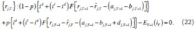
Replacing the reaction function for demand at the auction, j,T –1 , (21) in (22), we obtain reaction function for the reduction of the deficiency in T – 1, in terms of states (aj,T–1, rj,T–1), predetermined bj,T–1, exogenous Central Bank interest rates, and endogenous expectation on next-day interbank interest rate, ET–1(iT):
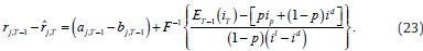
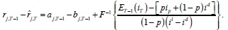
We replace reaction function for the reduction in the deficiency (23) in (21), and obtain reaction function for demand at the auction in terms of shock distributions, exogenous interest rates and endogenous expectation on next-day interbank interest rate, ET–1(iT):
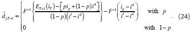
Again, like in T, it will prove to be useful to know how the auction's objective function at T – 1 changes with marginal supply of resources early in the day, when evaluated at the reaction function for the endogenous variables. We calculate:

Marginal reserves lent earlier in the day cost the expected value in T – 1 of the interbank interest rate in T. Note that at the equilibrium –see (14)– this expectation depends on the policy rate and size and sign of demand shocks in T.
2.3.2. Bank's Problem in the Interbank Market in Day t = T –1
Bank j optimizes over the value function:
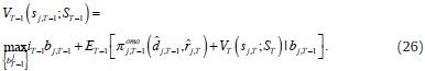
Value function in T – 1 has two arguments: profits in the interbank market and the expected value at the auction and next-period value function.
Equation (26) is a linear function in bj,T–1. Optimization can yield one of three options: a) iT–1> ET–1 (iT), where bank j would like to lend as much as possible in the interbank market at time T – 1; b) iT–1< ET–1 (iT), and bank j would like to borrow as much as possible from the interbank market, or c) iT–1= ET–1 (iT), where bank j would be indifferent between lending (or borrowing) today or tomorrow and we have infinite solutions for bTj –1, and all other endogenous variables that depend on it.
Assuming that bank j cannot lend in the interbank market more resources that the ones he has available at the time, the maximum amount he could lend would be [bj,T –1)max = aj,T –1. If this amount is positive for each and every bank, the situation iT–1= ET–1 (iT) cannot be an equilibrium since, in that case, bj,T –1>0, which violates the equilibrium condition in the interbank market. On the other hand, even if for some banks aj,T –1<0, those banks would not want to borrow today but tomorrow, and therefore, for them, bj,T –1=0. In conclusion, the event iT –1> ET –1(it) can be sustained as an equilibrium in the interbank market only if aj,T –1 ≤ 0, ∀j , so that b*j,T –1=0, ∀j.
In the event that iT–1< ET–1 (iT) bank j would like to borrow as much as possible from the interbank market. In principle, it would like to borrow rj,T, so that it covers its requirement already in T – 1. Bank j may want to borrow even more and put it in the deposit window at the Central Bank, obtaining a return of id. Because of the fact that in this event banks would like to borrow as much as possible to cover their deficiency and put resources in the deposit window at the central bank, it results that bj,T –1<0, and therefore the event iT–1< ET–1 (iT) can never be sustained as an equilibrium of the interbank market.
It can be concluded, then, that the only possible equilibrium for the interbank market is to have

We conclude that under this framework there are multiple (infinite) equilibria for the supply (or demand) of resources of bank j in the interbank market at time T - 1. According to equation (23), there are also multiple equilibria for the deficiency reduction. Furthermore, according to the interbank clearing market condition, in (5), there are multiple equilibria for the interbank interest rate (its expectation with conditional information at T - 1), demand at the auction and liquidity supply from the Central Bank.
The multiple equilibria is characterized by equation (23), where the more the commercial bank supply in the interbank market the less it can reduce its deficiency. There is a trade-off between the two objectives of maximizing profits in the interbank market and two objectives of maximizing profits in the interbank market and satisfying the requirement constraint. The bank has to choose along the linear relation in equation (23), how much it desires to supply (or demand) in the interbank market at time T - 1 with its correspondent reduction of the deficiency.
2.3.3. Determination of a Single Equilibrium
Supply at the interbank market and reduction of the deficiency are determined jointly. The commercial bank faces a trade-off according to equation (23): if it decides to reduce its deficiency, it sacrifices profits; and if it decides to supply at the interbank market and make profits, it does not reduces its deficiency and faces the risk of needing to accept more expensive liquidity.
We assume all institutions have preferences about how fast they want to reduce their deficiency. We propose W to represent those preferences. Bank j solves:

where 0 ≤ γj < ∞ is the relative weight that bank j gives to reducing its deficiency with respect to its benefits in the interbank market. Subject to equation (23):
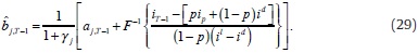
We replace (23) in (28) and use the Martingale result in (27). Then, first order condition gives reaction function for supply (or demand) of bank j in the interbank market in terms of the endogenous interbank interest rate in T - 1, states, exogenous variables and parameters:
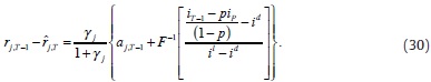
Replacing (29) in (23), again with the use of (27), we obtain reaction function for the reduction of the deficiency, also in terms of the endogenous interbank interest rate in T - 1, states, exogenous variables and parameters:
Replacing (29) in the clearing market condition in (5), we are able to solve for the equilibrium interbank interest rate in T - 1:
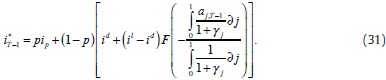
We replace (31) in equations (29) and (30), to find equilibrium supply (or demand) for resources in the interbank market and equilibrium reduction of the deficiency at time T - 1, respectively:
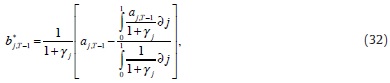
and
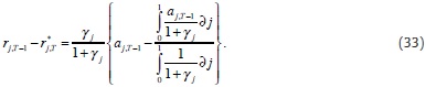
Equations (31) through (33) are the results of the model to be validated in section 3 of the paper. As we have noticed for time t = T, in time T – 1 equilibrium interbank interest rate is distorted by the uncertainty at the auction. The smaller the probability p of getting the liquidity demanded at the auction, the greater the distortion is. Once again, as in the last day of the requirement period, equilibrium liquidity supply by banks in the interbank market is not affected by the auction-window supply mechanism.
This result for T – 1, together with the equilibrium in T, indicates that the auction-window mechanism generates distortions with no benefits for the deepening of interbank activity. It is worth noticing that, as previously mentioned, the mechanism put in place might respond to other objectives different from the deepening of the interbank market which we do not consider or model in this paper.
2.4. Recurs iveness
Replacing equilibrium supply (or demand) of bank j in the interbank market (32) and equilibrium reduction of the deficiency (33) in the value function of day T – 1, (26), we calculate:

which is analogue to (18). Therefore, results for t = T – 1 can be iterated for all t ∈[1,T –1] .
3. Data Analysis
This section starts by describing the sources of information of Colombian interbank markets that are going to be used to validate the results (equilibria) of the model in section 2. Then, we focus on providing statistical evidence for the Martingale hypothesis, results at the last day of the requirement period and finally, for all other days.
3.1. Data
In order to show the patterns we find in Colombia data, we use information of the average reserve requirements and funds effectively held by banks, reported to the Colombian Regulator (Superintendencia Financiera [SF], form 443); interest rates and the amounts lent and borrowed by each bank in the uncollateralized market (SF, form 441); and interest rates and amounts traded in the collateralized interbank market from DCV (Depósito Central de Valores, Central Bank's depositary for clearing and delivering of Government bonds [TES]). This data includes records from SEN, MEC and those made OTC.
We focus our attention in analyzing and processing data for overnight operations only, and we find the global position in the interbank market for each bank (i.e., the amount lent in collateralized and uncollateralized markets minus the amount borrowed in both of them). We construct a weighted interest rate. The information about OMOs is taken from the Central Bank. We use the amounts demanded and actually obtained in the daily REPO auctions by each bank, and its corresponding interest rates. This information is used to calculate the supply shock (frequency of banks getting nothing out of the auction).
We build a database that reflects the operation of the monetary policy in Colombia. It contains money supply by the Central Bank and reserve requirements.
We consider all operations per entity, for each day of the period January 2012-April 2013. Our data base includes 34 full reserve requirement periods, which accounts for 57 596 observations.9 Because our purpose is to analyze all types of overnight operations among entities, which we called the total interbank market, we include the collateralized and non-collateralized transactions.10 From these operations, we exclude all transactions at rates lower than the deposit rate of the Central Bank because we recognize that those are for different purposes than the borrowing-lending type. With the remaining transactions, we define the following variables:
- Deficiency reduction: it corresponds to the daily value of the reserves for each institution. It does not include resources different from those used to meet reserve requirements.11 It is important to mention that not all entities considered here have to satisfy the reserve requirement (this is only for credit institutions).
- Total interbank interest rate: calculated as the weighted average of all collateralized and non-collateralized operations considered in the model.
- Daily operations with the Central Bank: REPO and window facilities net balance.
- Daily total interbank transactions: overnight collateralized and non-collateralized transactions. 57 596 observations resulted.
3.1.1. Parameters Used in the Data Analysis
In the results we show below, we calibrate values for supply and demand shock distribution parameters, and preference parameter γj in equation (28).
We assume that the demand shocks follows a logistic distribution function. Given that we have more than 50 000 observations, we assume that the sample mean and standard deviation correspond to their unobservable values. Therefore, we have a demand shock distribution with F(με =0,σε = 789.3 ) .
The supply shock follows a binomial distribution function with parameter p calibrated at 0.99. This parameter has been calculated from an average of the proportion of banks that, having participated in the auction, were given some liquidity.
Parameter capturing the preferences of banks over deficiency reduction and interbank activity γj was calibrated by dividing equations (29) and (30), using data by day and by bank, and then averaging by bank over the considered period.
3.2. The Martingale (Difference) Hypothesis
Equation (27) is an analytical derivation of the Martingale hypothesis proposed by PR (2006). In this section we aim to test whether the interbank interest rate follows this kind of process. We follow the method of Dominguez and Lobato (2003) to test Martingale difference hypothesis. From equation (27), we have

We use the definition of the conditional expectation to write.

which implies that the conditional expected marginal return of the interbank reserves is zero. The Martingale Difference Hypothesis allows us to claim that if equation (36) holds, the interbank interest rate follows a Martingale process.
We use the Dominguez-Lobato Test for Martingale Difference Hypothesis of the package: Variance Ratio tests and other tests for Martingale Difference Hypothesis, "vrtest", that runs in R, and was programmed by Kim (2011).12
The test sets
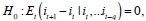
calculates de Cramer von Mises test statistic (Cp) and the Kolmogorov-Smirnov test statistic (Kp), with wild bootstrap p–value of the Cp test (Cp – pval) and wild bootstrap p–value of the Kp test (Kp – pval); with 300 bootstrap iterations, and q = 5 lags for the conditional expectation. This lag value was chosen because 5 is the average lag of a two-weeks maintenance period with 10 working days  ).
).
Results allow not to reject the null hypothesis with Cp = 0,0176; Kp = 0,5050; Cp – pval = 0,9367; Kp – pval = 0,8133.
Given that Cp – pval and Kp – pval are greater than 0,05, we do not reject the Martingale hypothesis process for the Colombian interbank rate.13
Economic meaning of a Martingale process might mean efficiency in the interbank market, because expected gains from one day to the next are statistically zero as all arbitrage possibilities have been taken. PR (2006) have come to set this hypothesis from their derivations, however to our understanding this is the first paper to produce a full analytical derivation of this result.
3.3. Model Results Versus the Interbank Mark et in Colombia
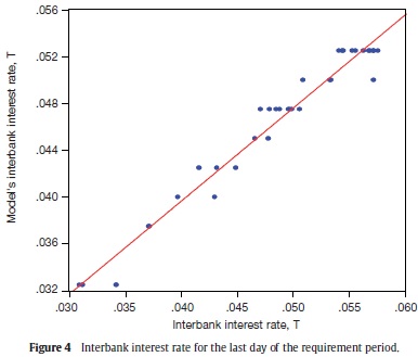
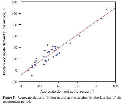
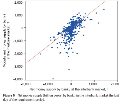
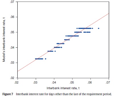
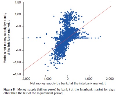
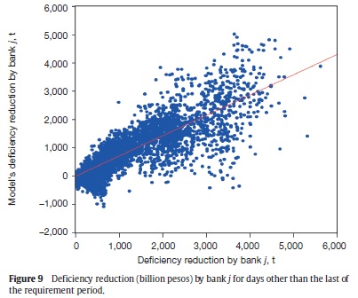
In this subsection, we present six scatter plots for variables of our interest where we compare observed data (always in the horizontal axis) with the model outcome (in the vertical axis). Each figure contains an OLS linear (with constant) regression line. In a perfect fit, one would get a 45° line (a coefficient of 1 in the linear regression). We present the regression results in the Appendix A.
We use equation (14) to obtain model's equilibrium interest rate of the interbank market for the last day of the requirement period. The model explains (adjusted R2) nearly 96% of the variable's variance, with a significant coefficient of 1.21, which means that our model underestimates this interest rate (Figure 4, and Table A1).
We use equation (16) to obtain model's equilibrium aggregate demand at auction for the last day of the requirement period. The model explains (adjusted R2) nearly 90% of the variable's variance, with a significant coefficient of 0.76, which means that our model overestimates the aggregate demand (Figure 5, and Table A2).
We use equation (15) to obtain model's equilibrium liquidity supply in the interbank market by bank j in the last day of the requirement period. The model explains (adjusted R2 ) nearly 35% of the variable's variance, with a significant coefficient of 0.25, which means that our model overestimates interbank activity (Figure 6, and Table A3).
We use equation (31) to obtain model's equilibrium interbank interest rate for days other than the last day of the requirement period. The model explains (adjusted R2 ) nearly 94% of the variable's variance, with a significant coefficient of 1.24, which means that our model underestimates this interest rate (Figure 7, and Table A4).
We use equation (32) to obtain model's equilibrium liquidity supply in the interbank market by bank j in days other than the last day of the requirement period. The model explains (adjusted R2) nearly 23% of the variable's variance, with a significant coefficient of 0.35, which means that our model overestimates this interbank activity (Figure 8, and Table A5).
We use equation (33) to obtain model's equilibrium reduction in the deficiency by bank j in days other than the last day of the requirement period. The model explains (adjusted R2) nearly 82% of the variable's variance, with a significant coefficient of 1.15, which means that our model underestimates the deficiency reduction (Figure 9, and Table A6).
4. Final Remarks
We have set a dynamic stochastic model for the interbank market in Colombia. We modify the structure of the model in PR (2006) in four aspects: first, we allow for daily auctions instead of one in the entire requirement period; second, we alter the timing of the model to have the auction after interbank trading has taken place, at any given day, and not before; third, the banks in our model optimally decide over the amount of reserves they accumulate each day to contribute to their reserve requirement, which is a residual in PR (2006). In this paper we present one of four possible timings for this decision to be made: simultaneously with the auction demand decision. Fourth, along with the demand shock in PR (2006), banks in our model face a second source of uncertainty: there is a probability of not obtaining resources at the auction, which is a shortcut for modelling an auction mechanism. Finally, the reader should note that our framework does not take into account frictions that would alter the perfect competition assumption, nor other sources of heterogeneity among institutions (e.g., size), neither risk perception between market participants (or other information problems).
We set two main objectives for the paper: first we aim to understand how interbank markets work, and second, how Central Banks mechanism to conduct monetary policy affects outcomes (interest rates and loans) in those markets. Even though we focus our attention in the Colombian case, the analytical tools we develop here can be used to study a wide range of interbank markets from different economies since they have some common features.
Our main findings are:
-
The equilibrium interbank interest rate is equal to the policy rate, ip, only if the probability of receiving the demanded resources at the auction is equal to one. Otherwise, the mechanism for money supply causes a distortion that separates the equilibrium interbank interest rate from the policy rate. The spread between these two rates depends on the size of the expected demand shocks, and is bounded by the rates at the Central Bank's facilities.
-
Optimal activity of bank j in the interbank market in the last day of the reserve period depends positively on its assets net of its deficiency, and aggregate demand for resources (aggregate deficiency net of aggregate assets). Equilibrium supply of resources in the interbank market the last day of the requirement period does not depend on the uncertainty of receiving resources at the auction. We conclude that, at least under the framework presented for the last day of the requirement period, the money supply mechanism with auction and window facilities does not encourage the deepening of the interbank market.
-
In days other than the last day of the requirement period, equilibrium interbank interest rate is distorted by the uncertainty at the auction. The smaller the probability of getting the liquidity demanded at the auction, the greater the distortion is. Once again, as in the last day of the requirement period, equilibrium liquidity supply by banks in the interbank market is not affected by the auction-window supply mechanism.
-
Overall results indicate that the auction-window mechanism generates distortion with no benefits for the deepening of interbank activity. It is worth noticing that, as previously mentioned, the mechanism put in place might respond to other objectives different from the deepening of the interbank market which we do not consider or model in this paper.
We are aware that our analytical results are conditional to the structure of the model presented in detail, in particular on the assumptions about the demand shock distribution and the supply shock modelling.
To our understanding, this paper is the first in presenting an analytical derivation for a Matingale process followed by the interbank interest rate. Economic meaning of a Martingale process might mean eficiency in the interbank market, because expected gains from one day to the next are statistically zero as all arbitrage possibilities have been taken.
Empirical analysis of our model's results regarding a Martingale process in the interbank interest rate is satisfactory: using Colombian data we test and do not reject the hypothesis that the interbank interest rate follows that kind of process. We also use the equilibrium equations of the model to validate our findings. We calibrate parameters γj and p and run linear regressions between the model estimations and Colombian data. In each of these seven regressions we place observed data in the left hand side of the regression and model estimations in the right hand side. Then, perfect fit of real data from the model would produce positive parameters which are statistically no different from one.
Thus, we produce estimations of the interbank interest rate, the interbank net supply of funds by bank at the interbank market and the deficiency reduction by bank for each day of the period considered (January 2012-April 2013). In addition, we estimate the aggregate demand at the Central Bank auction for the last days of the requirement period. The regressions results show that our model can explain near 95% of the variance in the interbank interest rate, near 80% of the variance in the deficiency reduction, and near 30% of the variance in the net money supply at the interbank market.
However, the model overestimates the interbank liquidity supply by banks, and underestimates the interbank interest rate and the deficiency reduction. We think that these results can be improved by modifying our analytical framework in three ways: first, it could be useful to constraint the model to have a positive reduction of the deficiency at all times; second, it could be useful to model other sources of heterogeneity among banks that capture risk factors, and third, it could be useful to analyze a case in which daily resources are not traded in the perfect competition fashion that we assume in our framework. We expect to explore these modifications in future research. We think that, in particular, constraining our model to have only positive reductions of the deficiency can solve some of the biases of the model results. With positive or null reduction of deficiency, banks need more liquid assets which should reduce net supply in the interbank market. This contraction of supply should produce a higher equilibrium interbank interest rate. Overall this change should improve the fit of the empirical exercises.
Acknowlegements
We thank two anonymous referees and ESPE editors José Eduardo Gómez and Jair Ojeda, as well as participants of the Research Agenda Seminar, the Macroeconomics Modelling Department Workshop, the Fedesarrollo weekly seminar, and the 10th Special edition of ESPE seminar for their very helpful comments and discussions. We thank Joaquín Bernal, Jesús A. Bejarano, Joaquín Coleff, Alexander Guarín, Carlos León, Julián A. Parra, Norberto Rodríguez, and Hector Zárate for very useful discussions, and Nicolás Camargo and Karen Quintana for research assistance.
Notes
1SEN stands for Sistema Electrónico de Negociación (Electronic Trading System) and is administrated by Banco de la República. On the other hand, MEC stands for Mercado Electrónico (Electronic Market) and it is administrated by the Colombian Stock Market (Bolsa de Valores de Colombia).
2Regulation allows the Central Bank of Colombia to hold expantionary and contractionary auctions for funds by REPOS.
3In the aggregate, the total interbank market is equal to zero. We show only one side of the transactions at the interbank market.
4We are aware that the timing of the decision about reserves may alter our results. Although we state that banks and banks-like institutions have an explicit strategy to fulfill their required reserve restrictions, we do not know when exactly this decision takes place during the day. In this paper we set the decision of how much the bank contributes to its reserve requirement with the auction, and let other configurations for further research.
5Reduction in the deficiency should be non-increasing to reflect Colombian regulation (i.e., rj,t – rj,t+1 ≥ 0). We do not attempt to incorporate this feature in this paper to keep the algebra tractable.
6Throughout the paper we refer to the auction as if it were an expantionary mechanism; however, Colombia regulation allows for contractionary auctions, and in the model it is posible to obtain dj,t< 0.
7It is useful to see it this way: bank j started day t with αj,t. It gave away resources at the interbank market (bj,t), received dj,t at the auction with probability p, and the demand shock εj,t. Next day, the bank recovers what it lent and pays back the money demanded at the auction. Therefore, it starts the next day with assets: αj,t+1 = mj,t+ εj,t+ + bj,t – dj,t= αj,t + εj,t.
8In particular, demand shock in T – 1 determines liquid assest at time T, and endogenous decision about reduction of deficiency in T – 1 determines rj,T.
9In Colombia, a reserve requirement period includes a total of 14 days, starting a Wednesday and finishing a Tuesday two weeks later. During this period, the amount held as reserves every day (including weekends) is considered in the average for the reserve requirement.
10In this sense, our goal is not to explain the interbank interest rate market as it is usually understood. Usually interbank or overnight rate is the rate resulting from non-collateralized transactions among entities. As we mentioned before, our interest is to analyze these operations along with those that are collateralized. Therefore, the resulting average rate of both types of transactions is what we call total interbank interest rate.
11It does not include resources kept in deposit or lending facilities at the Central Bank.
12See reference in Charles et al. (2011).
13Code in R is available at the request of the reader.
References
Casella, G., Berger, R.L. (1990). Statistical Inference. Duxbury, Belmont. p. 69. [ Links ]
Cardozo, P., Huertas, C., Parra, J., Patiño, L. (2011). Mercado interbancario colombiano y manejo de la liquidez del Banco de la República. Borradores de Economía, 673. [ Links ]
Charles, A., Darne, O., Kim, J.H. (2011). Small sample properties of alternative tests for Martingale Difference Hypothesis. Economics Letters, 110, 151-154. [ Links ]
Dominguez, M.A., Lobato, I.N. (2003). Testing the Martingale Difference Hypothesis. Econometric Reviews, 22, 351-377. [ Links ]
Freedman, C., Laxton, D. (2009). Why inflation targeting? IMF Working Paper/09/86. [ Links ]
González, C. (2013). Mercados interbancarios no colateralizados e información asimétrica. Borradores de Economía, 758. Banco de la República de Colombia, Bogotá [ Links ].
Jurgilas, M. (2006). Interbank markets under currency boards. Working papers 2006-19, University of Connecticut, Department of Economics. [ Links ]
Kempa, M. (2006). Money market volatility. A simulation study. Research Discussion Papers 13/2006, Bank of Finland. [ Links ]
Kempa, M. (2007). What determines commercial banks' demand for reserves in the interbank market. Research Discussion Papers 30/2007, Bank of Finland. [ Links ]
Moschitz, J. (2004). The determinants of the overnight interest rate in the euro area. Working Paper Series 393, European Central Bank. [ Links ]
Pérez Q.G., Rodríguez M. (2006). The daily market for funds in Europe: What has changed with the EMU? Journal of Money, Credit and Banking, 38, 91-118. [ Links ]
Pérez Q.G., Rodríguez M. (2010). Asymmetric standing facilities: an unexploited monetary policy tool. Working Papers 1004. Banco de España, Madrid. [ Links ]
Appendix A Regression Results
