An Early Warning Model for Predicting Credit Booms Using Macroeconomic Aggregates^*

Un modelo de alerta temprana para la predicción de booms de crédito usando los agregados macroeconómicos

Alexander Guarín^a,**, Andrés González^a, Daphné Skandalis^a, and Daniela Sánchez^a

^* The opinions expressed here are those of the authors and do not necessarily represent neither those of the Banco de la República nor of its Board of Directors. As usual, all errors and omissions in this work are our responsibility.
^a Banco de la República, Bogotá, Colombia

^** Corresponding author. E-mail address: aguarilo@banrep.gov.co (A. Guarín).

ABSTRACT

In this paper, we propose an alternative methodology to determine the existence of credit booms, which is a complex and crucial issue for policymakers. In particular, we exploit the Mendoza and Terrones's (2008) idea that macroeconomic aggregates contain valuable information to predict lending boom episodes. Specifically, our econometric method is used to estimate and predict the probability of being in a credit boom. We run empirical exercises on quarterly data for six Latin American countries between 1996 and 2011. In order to capture simultaneously model and parameter uncertainty, we implement the Bayesian model averaging method. As we employ panel data, the estimates may be used to predict booms of countries which are not considered in the estimation. Overall, our findings show that macroeconomic variables contain relevant information to identify and to predict credit booms. In fact, with our method the probability of detecting a credit boom is 80%, while the probability of not having false alarms is greater than 92%.

Keywords: Early warning indicator, Credit booms, Bayesian Model Averaging, Emerging markets.

JEL Classification: E44, E52, G21, E32, E37, E44, E51, C53.

RESUMEN

En este documento se propone una novedosa metodología para determinar la existencia de booms de crédito, el cual es un tema bastante complejo y de crucial importancia para las autoridades económicas. En particular, se explota la idea de Mendoza y Terrones (2008) que señala que los agregados macroeconómicos contienen información valiosa para predecir los episodios de boom. El ejercicio econométrico realiza la estimación y predicción de la probabilidad de estar en un boom de crédito. El trabajo empírico se lleva a cabo a partir de datos trimestrales de seis países latinoamericanos entre 1996 y 2011. Para capturar simultáneamente la incertidumbre en la elección del modelo y el valor de los parámetros, se emplea la técnica Bayesian Model Averaging. Como se hace uso de datos panel, los resultados econométricos podrían ser empleados para predecir booms de países que no se consideran en la estimación. En conjunto, los resultados muestran que las variables macroeconómicas contienen información importante para identificar y predecir los booms de crédito. De hecho, con nuestro método la probabilidad de detectar un boom de crédito es 80% mientras la probabilidad de no tener falsas alarmas es mayor al 92%.

Palabras clave: Indicador de Alerta temprana, Booms de Crédito, Promedio Bayesiano de Modelos, Mercados Emergentes.

Clasificación JEL: E32, E37, E44, E51, C53.

1. Introduction

In general, a credit boom is defined as an excess of lending above its long-run trend. Credit booms tend to make economies more volatile and vulnerable, and are often associated with increases in inflation, declines in lending standards, instability in the banking sector and increases in the probability of financial crisis (Reinhart and Kaminsky 1999; Gourinchas et al., 2001; Barajas et al., 2007, Dell'Ariccia et al., 2012, and Williams, 2012). Consequently, the identification of episodes of credit boom and their early prediction is a crucial problem for policymakers.

Nevertheless, the correct determination of these booms is a complex problem that is far from being straightforward in practice. Recent literature on credit booms characterizes these latter as periods where the cyclical component of lending exceeds a specific threshold, and associates these episodes with the dynamics of macroeconomic aggregates (e.g. Gourinchas et al., 2001; Cottarelli et al., 2005; Kiss et al., 2006, and Mendoza y Terrones, 2008). However, these works do not focus on the construction of early warning indicators of credit booms.

The main objective of this paper is the construction of a quantitative tool that allows the identification and early prediction of credit boom episodes by exploiting the relationship between these latter and the macroeconomic aggregates. Our indicator is based on two elements: the probability of being in a credit boom at time t + h for h ≥ 0 conditioned on the set of data available at time t, and second, on an estimated threshold value that establishes the probability at which the model defines the existence of a credit boom.

The probabilities of credit boom are computed through a Bayesian average of many logistic regression models applied to panel data. The Bayesian model averaging (BMA) methodology deals with both parameter and model uncertainty. In our case, model uncertainty is related to the selection of the macroeconomic aggregates that should be included as explanatory variables in the logistic regression. The BMA runs a large number of estimates on different combinations of covariates, and then, takes the weighted average of all the results. The weights are given by the model posterior probability.

The econometric analysis is applied on quarterly data of six Latin American countries between 1996 and 2011. Our findings show that macroeconomic aggregates hold valuable information to identify lending boom episodes and to provide early warning signals about future booms. The estimated probabilities of being in a credit boom at time t + h with h ≥ 0 show an outstanding performance. For instance, in our sample of Latin American countries, we estimate a threshold probability of 38%, which implies a probability of detecting a credit boom of 80.3% and a probability of not having false alarms greater than 92%.

In order to test whether macroeconomic variables provide additional information to the credit growth rate in the identification of credit boom episodes, we run the BMA algorithm on two sets of covariates. The first set only considers macroeconomic aggregates as explanatory variables in the model while the second set additionally includes the credit growth rate.

We also carry out a cross-validation exercise across countries to check the reliability of our results. Our findings indicate that the determinant factors of credit booms are similar across countries, and that those factors can be captured with standard macroeconomic variables. These results also suggest that our algorithm may be used to predict lending booms of countries in the region that are not considered in the estimation and that may have short time series data.

Overall, this paper provides a valuable tool to quantify the probability of being in a credit boom, or having a boom in the future. To the best of our knowledge, this is the first paper that performs the estimation and prediction of credit boom probabilities using macroeconomic data. In this sense, both the methodology and the empirical results for our sample of Latin American countries represent a new contribution to the burgeoning literature on credit booms.

The reminder of this paper is organized as follows. Section 2 presents the econometric methodology. Section 3 goes into the details of the data set used in the empirical exercise. In Section 4 we perform the empirical exercises. Finally, Section 5 brings some conclusions.

2. Econometric Methodology

In order to estimate the probability of credit boom, we use the logistic regression model with panel data and fixed effects

where y_i,t+h = 1 if there is a credit boom for country i at quarter t + h, h ≥ 0 and y_i,t+h = 0 otherwise, β is a R × 1 parameter vector, ε_it is the error term and x_it = (x_1,it, ..., x_R,it) is a set of R covariates, α_i with i = 1, ..., I are the fixed effects.

Our aim is to estimate the probability of being in a credit boom at time t + h with h ≥ 0 conditioned on the information at time t through the following equation

where F is the cumulative logistic distribution function and θ = [α'β'] ' with α = [α₁, ..., α_I]'.

In order to deal simultaneously with the model and the parameter uncertainty, we apply the BMA methodology (see Raftery, 1995, and Raftery et al., 1997). We assume that M = [M₁, ..., M_k] is the set of all models, where M_k is the k-th model, which is defined by the subset of covariates included in the model, and whose size is less or equal to R.

The BMA probability of being in a credit boom at time t + h, h ≥ 0 is given by

where p(θ^k,M_k |D) is the joint posterior probability,θ^k is its associated parameter vector and D denotes the data set. As can be seen, the BMA probability in equation (3) is a weighted average of equation (2) where the weights are given by p(θ^k,M_k |D). Since the joint posterior probability is unknown, we approximate equation (3) using the reversible jump Markov chain Monte Carlo (RJMCMC) algorithm introduced by Green, 1995 (see also Hoeting et al., 1999; Brooks et al., 2003, and Green and Hastie, 2009, for additional details).

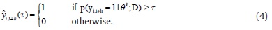
Even though the probability p^BMA(γ_i,t+h= 1| D) is informative, it is interesting to determine a value of this probability at which we have a clear warning of the existence of a credit boom. In other words, how large does this probability need to be before calling for a credit boom? To answer this question, we define a threshold value, τ ∈ [0,1], over which the methodology defines the warning. This estimation is carried out through a variable _i,t+h (τ) defined as

Note that for a given probability p(yi,t+h = 1|θ ^k ;D), the number of estimated credit booms depends on the threshold τ. If this latter is very small, then we will have many warnings of credit boom which could be false alarms. On the contrary, if τ is very large, then we will have few warnings, and the probability of having undetected booms would be larger.

In order to define a threshold probability, we compute the value τ that

Min ø(τ) subject to γ(τ) ≤

where ø (τ) is the proportion of credit boom's false alarms, γ (τ) is the proportion of undetected credit booms and is the maximum value of γ admitted by the policymaker. The values of γ (τ) and ø (τ) are estimated as

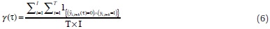
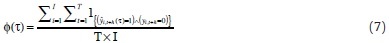
for h ≥ 0, where 1_{·} is an indicator variable equal to 1 if condition {·} is satisfied, and 0 otherwise. The quantity T × I stands for the total number of observations in the sample.

3. Data: C redit Booms and Macroeconomic Aggregates

We use quarterly data from Argentina, Brazil, Chile, Colombia, Mexico and Peru between the first quarter of 1996 and the fourth quarter of 2011. Our set of covariates includes the contemporary value and the first three lags of the macroeconomic aggregates highlighted by Mendoza and Terrones, 2008, as relevant to determine credit booms: domestic economic activity variables (Gross Domestic Product [GDP], investment, private consumption and government spending), international trade variables (exports, imports, terms of trade [ToT], real exchange rate [RER], current account), and financial system variables (asset prices and net capital flows)¹. This set considers in overall 44 covariates. The lagged values of the explanatory variables are included in order to capture the build up process of credit booms over time. In specific exercises, we additionally include the quarterly growth rate of the per-capita real credit and its first three lags. This new set considers 48 covariates.

Data come from the International Monetary Found (IMF) and Central Banks websites². The covariates: GDP, investment, private consumption, government spending, exports, imports and asset prices are seasonally adjusted and expressed in real terms through the consumer price index (CPI). The RER corresponds to national currency units for special drawing rights (SDR) of the IMF basket expressed in real terms with the CPI. The ToT are defined as the ratio between the prices of exportable and importable goods. We compute the cyclical component of these variables with the Hodrick-Prescott filter³. Current account and net capital flows are percentages of GDP. These variables are smoothed out with a non-centered moving average of order two.

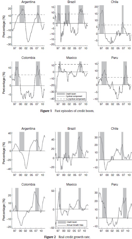
To compute credit boom episodes, y_i,t+h, we follow Mendoza and Terrones, 2008. That is, y_i,t+h = 1 when the cyclical component of credit⁴ is greater than one standard deviation of its historical measure, and y_i,t+h = 0 otherwise. We compute the cyclical component of per-capita real credit using credit data from domestic financial and depositary institutions to the private sector. The credit variable is expressed in per-capita terms using the working age population and deflated using the CPI. The cyclical component of credit is also calculated with the Hodrick-Prescott filter. Table 1 summarizes the dates of lending booms. Figure 1 shows credit boom episodes (gray areas) for the countries in our sample between 1996 and 2010.

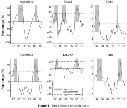
Figure 1 and Table 1 show an average of two credit boom episodes in our sample for each country. In fact, we note that booms are clustered in two well defined periods, but their specific dates and their duration vary across countries. The first period runs between 1997 and 2002. Credit boom episodes of this cluster are generally associated to the process of financial liberalization, privatization, opening to the international competition and the financial deepening of the region during the nineties (see Smith et al., 2008). Furthermore, these booms preceded the recession periods and financial crises observed in some countries of the region (e.g. Colombia in 1999 and Argentina in 2002). The second cluster includes lending booms detected between 2007 and 2008, which preceded the recent credit crunch and the international financial crisis.

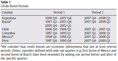
Figure 2 shows the relationship between the dynamics of the annual credit growth rate (black line) and the periods of credit boom (gray area). This figure supports the argument by Terrones and Mendoza, 2004, that lending boom episodes happen less often than periods of fast credit growth because these latter are affected by the economic cycle. Terrones and Mendoza, 2004, also argue that the credit growth rate is not a sufficient indicator of credit booms because periods of high growth rates can be the result of other situations such as financial deepening processes or episodes of catching up after recessions. This could be the case in Mexico, which undergoes a large expansion of credit at the end of 2002 and at the beginning of 2003, but does not suffer from a credit boom in those periods. Moreover, most of the time credit booms start once the credit growth rate has reached its maximum value. See, for example, credit booms in Colombia and Argentina that start when their credit growth rate was already declining.

4. Empirical Analysis

This section presents the estimated and predicted probabilities⁵ of being in a credit boom at time t + h, h = 0,1,2 defined in equation (3). The full sample defined in Section 3 is divided in two parts. The first set [x_it, y_i,t+h] corresponds to data between the first quarter of 1996 and fourth quarter of 2010. Unless otherwise indicated, this set of data is used to carry out the estimation of BMA parameters and in-sample estimates of probabilities of lending boom. The second part of the sample only considers data of macroeconomic aggregates during 2011, x_it. These data are used to perform both ex-ante and ex-post out-of-sample forecastings⁶ of probabilities of credit boom.

The threshold probability τ is computed by solving the minimization problem (5) with a maximum value of undetected credit booms equal to 5 percent of the observations in our sample.

The first exercise computes the BMA probabilities described by equation (3) for h = 0, when there are no fixed effects, α_i = α, and the set x_it does not include information of the credit growth rate. Figure 3 shows the estimated (thin line) and ex-post predicted (thick line) probabilities. From now on, the gray areas correspond to periods of credit boom previously identified in Section 3. The threshold probability (dashed line) is estimated at 37%. This figure exhibits an excellent fit of the estimated probability regarding to the established credit booms. For instance, periods of boom show high values of the estimated probability. On the contrary, the estimated probability is close to zero when there is no a boom. In fact, the probability of detecting a credit boom is 79%, while the probability of not having false alarms is 90%.

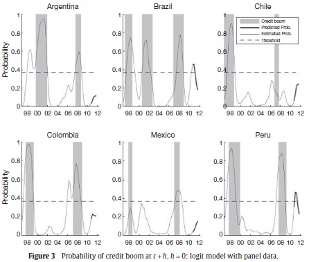
As can be seen in Figure 3, our method captures most of the episodes of credit boom, except for the first episode of Mexico in 1998 and the second boom of Chile in 2007. These undetected booms can be the result of a failure of our methodology, or simply, the Mendoza and Terrones, 2008, method makes a wrong identification of these periods as credit booms. In fact, the first episode in Mexico may be the result of a catching up process after the financial crisis in 1995 rather than a lending boom.

The outstanding performance of the estimated probabilities suggests that the macroeconomic aggregates of the countries in our sample contain valuable information to identify and to predict credit boom episodes. Figure 3 shows that the predicted probability of being in a credit boom increases for all countries between the first and fourth quarter of 2011. However, only for Brazil and Peru the predicted probabilities are larger than the threshold value.

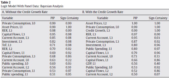
Our algorithm also provides some lights on the main driving macroeconomic forces of credit booms. Table 2 reports the posterior

inclusion probability (PIP)⁷ and the sign certainty. The PIP stands for the probability that an explanatory variable is included in the model. The sign certainty presents the probability that the estimated coefficient is positive. We denote the contemporary value and the first three lags of the variable (·) as L0, L1, L2 and L3. Panel A in Table 2 shows the statistics for the covariates with the highest PIP values for the model without credit growth rate as explanatory variable. According to the PIP, the most important variables in the estimation are private consumption (L0, L3, L1), asset prices (L1), RER (L3,L2), capital flows (L3, L1) and current account (L3,L0). The increase of the capital flows to GDP ratio and the cyclical component of private consumption and asset prices have a positive effect on the probability of being in a credit boom. On the contrary, the increase in the cyclical component of the RER and the current account to GDP ratio reduce that probability.

In order to provide evidence on the robustness and reliability of the out-of-sample forecastings, we repeat the previous exercise with a new definition of the periods of estimation and forecasting. The former considers data between the first quarter of 1996 and fourth quarter of 2006, while the latter is defined between the first quarter of 2007 and the fourth quarter of 2011. Appendix B describes in detail the characteristics of this exercise and presents its results. Although the new in-sample estimation period only includes the first set of credit booms defined in Table 1, the ex-post out-of-sample forecasting of the BMA probability is able to capture most of the credit boom episodes between 2007 and 2008. In fact our methodology forecasts the second booms of Colombia and Peru and the third boom of Brazil.

We also carry out a cross-validation exercise across countries. In this exercise, we take out the data of country i (i.e. the dummy variable y_it and the covariates x_it), and estimate the BMA probability described in equation (3) with the remaining data. Once the estimation is performed, we compute the BMA probabilities of being in a credit boom for country i using the observed values of the variables x_it for that country. The estimation is carried out for each t between the first quarter of 1996 and the fourth quarter of 2010. The routine is performed for each country in our sample.

Figure 4 shows the BMA estimated probability (black line) of the cross-validation exercise. Each panel plots the computed probability for the country that is not included in the estimation. For instance, the panel with the label Argentina contains the computed probability for Argentina when no data for this country was used in the BMA algorithm. The probabilities in Figure 4 fit very well the episodes of boom already established. Moreover, these results agree in general with the estimated probabilities in Figure 3. The panel data structure in this econometric exercise allows to use the estimated parameters to compute the probabilities of being in a credit boom episode in countries of the region which are not considered in the estimation.

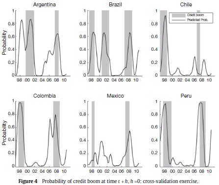
The findings of this exercise suggest that the determinant factors of credit booms are similar across countries, and that those elements can be captured by the evolution of the macroeconomic aggregates.

The most relevant common factors in the BMA estimated probability in the cross-validation exercise are the cyclical component of both the private consumption and asset prices, and the ratios of capital flows/GDP and current account/GDP. These results are in line with the recent literature on the causes behind credit boom episodes in emerging economies, and specially, Latin American countries. In particular, this literature points out the importance of capital flows on the deterioration in the loan-quality, the increase in government spending and the formation of both lending booms and asset price bubbles (Gavin and Hausmann, 1996; Ostry, 2007; Furceri et al., 2011; Montoro and Rojas-Suarez, 2012, and Montiel, 2013).

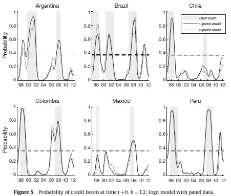
In order to assess the usefulness of our method as an early warning indicator of credit booms, we compute the BMA probabilities for h = 1,2 and α_i = α. Figure 5 shows the estimated BMA probabilities for h = 1 (thin black line) and h = 2 (thin gray line). The ex-ante predictions (thick lines) for h = 1,2 are also drawn. The threshold for h = 1 (black dashed line) and h = 2 (gray dashed line) are estimated in 37.3% and 35.9%, respectively. Under this setting, the probabilities of detecting a credit boom at time t + 1 and t + 2 are 80% and 79.8%, while the probabilities of not having false alarms are 90.6% and 90.4%, respectively. Consequently, our method can be used to anticipate credit booms at least six months in advance. The performance of this methodology, as an early warning indicator, depends on each country and the horizon h. For example, the predicted probabilities accurately anticipate all booms in Argentina, Colombia, Peru and the second booms in Brazil and Mexico. However, our method fails to anticipate Mexico's first boom and Chile's second one. The remaining booms are anticable 1pated but their time warning is very small.

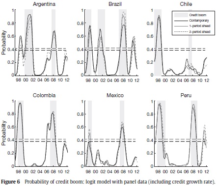
To see if the growth rate is a sufficient indicator of current or future credit booms, we repeat the econometric exercise but this time we include the credit growth rate within the explanatory variables. Figure 6 shows the estimated (thin line) and predicted (thick line) probabilities. The results are presented for h = 0 (black line), h = 1 (dark gray line) and h = 2 (light gray line). As can be seen in Figure 6, the fit is enhanced when the credit growth rate is included. We estimate a threshold of 38% (dashed line) that implies a probability of detecting a credit boom of 80.3% and a probability of not having false alarms of 92%. These values are higher than those found using only the set of macroeconomic aggregates. Moreover, the estimated boom probabilities when h = 1,2 exhibit a better anticipation of the lending boom events. Unlike the results presented for the model without credit growth rate, this new exercise weakly detects Mexico's first credit boom. Furthermore, the estimated probabilities for the second booms of Argentina, Colombia and Mexico are higher.

Panel B in Table 2 reports the PIP and the main statistics of this BMA estimation for h = 0. These results show that macroeconomic aggregates are still relevant in the estimation. In fact, variables with the highest PIP are asset prices (L2), private consumption (L0, L3), credit growth rate (L3), RER (L3) and current account (L3, L0). These covariates and their sign agree with those of the previous econometric exercise. Nevertheless, capital flows are not as relevant as before.

Appendix C reproduces the econometric exercise for the logistic regression model with fixed effects. The results in Appendix C are very similar to those reported here. Perhaps, the most interesting results are that the estimated and predicted probabilities for Argentina, Colombia and Mexico are, in general, lower in the model with fixed effects. On the contrary, the same probabilities for Brazil are higher. This result suggests that the characteristics of the Brazilian economy lead to a credit boom probability that is on average higher than in the rest of the region. This increase in the average probability is captured by the other countries when the model without fixed effects is considered.

5. Conclusions

In this paper, we present a novel methodology to identify and predict credit boom episodes based on macroeconomic aggregates. We show that this econometric method works as an early warning tool on the building up of lending booms, and hence, it can be used for policymakers.

Our findings show that macroeconomic variables provide valuable information to determine the existence of credit booms and to give early warning signals on the construction of new ones. Moreover, our results suggest that the determinant factors of these boom episodes across countries are similar, and therefore, our estimates can be used to predict booms of countries that are not considered in our sample. Even if the credit growth rate is included as explanatory variable, the macroeconomic variables remain relevant to estimate and predict lending boom episodes.

The results show that the estimated probabilities of credit boom achieve a very good fit for episodes previously determined by Mendoza and Terrones's, 2008, methodology. Nevertheless, if the credit growth rate is added to the set of covariates, the fit is enhanced.

Acknowledgements

We would like to express our gratitude to Hernando Vargas and Sergio Ocampo for their valuable comments and suggestions and to Camila Fonseca for their assistance in the research work.

Notes

¹Our set of covariates does not include the interest rate. The main reason is that this variable is very volatile during some short periods of time in our sample, which affects the identification of episodes of credit boom. For instance, the lending interest rate for Argentina between the first and third quarter of 2002 increased by 60% and then, reduced 48% in the fourth quarter of the same year. Brazil reduced its lending interest rate by more than 38% between the first quarter of 1999 and 2000.

²Appendix A summarizes the set of covariates included in this research, the definition of each one and its specific source.

³This filter uses a parameter λ=1600, which is standard in the literature for data with quarterly frequency. In order to check the sensitivity of results regarding the chosen filter and its parameterization, we perform two exercises. The first one considers the Hodrick-Prescott filter for several values of λ, while the second one is associated to the chosen filter (i.e. Christiano-Fitzgerald and Butterworth filters). These exercises show that results are insensitive to small variations of λ in the Hodrick-Prescott filter. On the contrary, identified periods of credit booms present relevant changes if the variations of λ are large or if we use other filters.

⁴Note that this measure is computed on the level of the variable and not on its growth rate.

⁵The BMA estimates are performed through a Markov chain with one hundred and twenty thousand draws. The first twenty thousand estimates are burned-up to avoid the noise in the choice of the initial seed. We assume that the prior model probability is , for all k = 1, ... , K, and the prior distribution of θ^k is N (0^k, 100 · I^k) where the zero vector 0^k and the identity matrix I^k change of size with the model M_k.

⁶The ex-ante forecastings correspond to predictions of p(y_i,t+h = 1|θ; x_it) for h > 0. The probabilities of credit boom at time t + h , h = [1,2] are predicted using data of covariates x_i available up to time t. On the other hand, the ex-post forecasting considers the predictions of p(y_i,t+h = 1|θ; x_it) for h = 0. The information of variables x_i from period t + 1 are used to predict t + h outcomes for the model estimated.

⁷7. The PIP is defined as 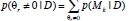where p stands for the probability, θ_r is the r-th element of the parameter vector θ, r = 1,..., R indexes el set of parameters, R is the total number of covariates and D denotes the data set. The variable M_k represents the k-th model, k = 1,..., K indexes the set of selected models and K is the total number of models.

References

Barajas, A., Dell'Ariccia, G., Levchenko, A. (2007). Credit Booms: The Good, The Bad and The Ugly. Manuscript, IMF.         [ Links ]

Brooks, S., Friel, N., King, R. (2003). Classical Model Selection Via Simulated Annealing. Journal of The Royal Statistical Society 65, 503-520.         [ Links ]

Cottarelli, C., Vladkova, I., Dell'Ariccia, G. (2005). Early Birds, Late Risers, and Sleeping Beauties: Bank Credit Growth to The Private Sector in Central and Eastern Europe and in The Balkans. Journal of Banking & Finace 29, 83-104.         [ Links ]

Dell'Ariccia, G., Igan, D., Laeven, L. (2012). Credit Booms and Lending Standards: Evidence From The Subprime Mortgage Market. Journal of Money, Credit and Banking 44, 367-384.         [ Links ]

Furceri, D., Guichard, S., Rustecelli, E. (2011). Episodes of Large Capital Inflows and the Likelihood of Banking and Currency Crises and Sudden Stops. Working Paper 865, OECD Economics Department.         [ Links ]

Gavin, M., Hausmann (1996). The Roots of Banking Crises. The Macroeconomic Context. In: L. Rojas-Suarez (ed.), Banking Crises in Latin America. John Hopkins University Press, Baltimore.         [ Links ]

Gourinchas, P., Valdes, R., Landerretche, O. (2001). Lending Booms: Latin America and The World. Working Paper 8249, NBER.         [ Links ]

Green, P. (1995). Reversible Jump Markov Chain Monte Carlo Computation and Bayesian Model Determination. Biometrika 82, 711-732.         [ Links ]

Green, P., Hastie, D. (2009). Reversible Jump MCMC. Genetics 155, 1391-1403.         [ Links ]

Hoeting, J., Madigan, D., Raftery, A., Volinsky, C. (1999). Bayesian Model Averaging: A Tutorial. Statistical Sciencie 14, 382-417.         [ Links ]

Kiss, G., Nagy, M., Vonnák, B. (2006). Credit Growth in Central and Eastern Europe: Convergence or Boom? Working Paper 2006/10, The Central Bank of Hungary.         [ Links ]

Mendoza, E., Terrones, M. (2008). An Anatomy of Credit Booms: Evidence From Macro Aggregates and Micro Data. Working Paper 14049, NBER.         [ Links ]

Montiel, P. (2013). Capital Flows: Issues and Policies. IDB-WP 411, Inter-American Development Bank.         [ Links ]

Montoro, C., Rojas-Suarez, L. (2012). Credit at Times of Stress: Latin American Lessons from the Global Financial Crisis. Woking Paper 370, Bank for International Settlements.         [ Links ]

Ostry, J. (2007). Managing Capital Flows: What Tools to Use? Asian Development Review 29, 83-89.         [ Links ]

Raftery, A. (1995). Bayesian Model Selection in Social Research. Sociological Methodology 25, 111-164.         [ Links ]

Raftery, A., Madigan, D., Hoeting, J. (1997). Bayesian Model Averaging for Linear Regression Models. Journal of The American Statistical Association 92, 179-191.         [ Links ]

Reinhart, C., Kaminsky G. (1999). The Twin Crises: The Causes of Banking and Balance of Payments Problems. The American Economic Review 89, 473-500.         [ Links ]

Smith, J., Juhn, T., Humphrey, C. (2008). Consumer and Small Business Credit: Building Blocks of The Middle Class. In: Haar, J., Price, J. (eds.), Can Latin America Compete? Confronting The Challenges of Globalization. Palgrave Macmillan.         [ Links ]

Terrones, M., Mendoza, E. (2004). Are Credit Booms in Emerging Markets A Concern? In: World Economic Outlook. Chapt. IV. IMF, Washington. pp. 147-166.         [ Links ]

Williams, G. (2012). Beyond the Credit Boom: Why Investing in Smaller Companies is Not Only Responsible Capitalism but Better for Investors Too. Working Paper 2012/02, The Institute for Public Policy Research.         [ Links ]

Anexo A

Anexo B

Anexo C