http://dx.doi.org/10.1016/j.espe.2014.10.001

Banking fragility in Colombia: An empirical analysis based on balance sheets^*

Fragilidad bancaria en Colombia: Un análisis basado en las hojas de balance

Ignacio Lozano^a,*, Alexander Guarín^b

^a Banco de la República (Central Bank of Colombia), Colombia

^* This paper benefited from the valuable comments of an anonymous referee. The authors would like to express our gratitude to Aura García for her exceptional assistance in this research work, and to Camila Londono, Diego Martinez and Javier Beltrán for their help in handling databases. The opinions expressed here are those of the authors and do not necessarily represent neither those of the Banco de la República nor of its Board of Directors. As usual, all errors and omissions in this work are our responsibility.

^** Corresponding author. E-mail address: ilozanes@banrep.gov.co (I. Lozano).

Article history:
Received 23 July 2014 Accepted 8 October 2014 Available online 11 November 2014

ABSTRACT

In this paper, we study the empirical relationship between credit funding sources and the financial vulnerability of the Colombian banking system. We propose a statistical model to measure and predict banking fragility episodes associated with credit funding sources classified into retail deposits and wholesale funds. We compute the probability of financial fragility for both the aggregated banking system and the individual banks. Our approach performs a Bayesian averaging of estimated logit regression models with monthly balance sheet data between 1996 and 2013. The results show the increasing use of wholesale funding to support credit expansion is a potential source of financial fragility. Therefore, monitoring credit funding sources could provide an additional tool to warn against banking disruptions.

Keywords: Credit cycle, Financial stability, Balance sheet, Logistic model regression, Bayesian model averaging.

JEL classification: C11, C23, C52, C53, G01, G20, G21.

RESUMEN

En este documento se estudia la relación empírica entre las fuentes de fondeo del crédito y la vulnerabilidad financiera del Sistema Bancario Colombiano. El trabajo propone la estimación Bayesiana de modelos de regresión logística para identificar y predecir episodios de fragilidad bancaria asociados con las fuentes tradicionales y no tradicionales de fondeo, que utilizan los bancos para proveer crédito. En particular, el ejercicio estima la probabilidad de que se presenten eventos de fragilidad tanto para el sistema bancario agregado como para los bancos individuales con datos mensuales de las hojas de balance para el periodo 1996-2013. Los resultados muestran que el creciente uso de los recursos no tradicionales para fondear el crédito, especialmente en sus fases de expansión, son fuente potencial de fragilidad financiera. Por consiguiente, el monitoreo a dichos recursos, a través de la técnica propuesta, proporciona una herramienta para detectar esos eventos.

Palabras clave: Ciclo del crédito, Estabilidad financiera, Hoja de balance, Modelo de regresión logística, Promedio Bayesiano de modelos.

Códigos JEL: C11, C23, C52, C53, G01, G20, G21.

1. Introduction

Since the beginning of the global economic crisis in mid-2007, topics concerning financial stability have gained importance in both the theory and the practice of macroprudential policy. An understanding of issues such as the funding structure of bank lending, the role of leverage, the determinants of credit cycles and the identification of credit booms have become crucial subjects for authorities, given their aim of anticipating and avoiding financial crises. These themes are particularly relevant in emerging economies where periods of rapid expansion in credit could arise diverse fragilities in the financial system.

Literature on financial stability has studied extensively the dynamics of credit, the measurement of the financial cycle and its relationship to banking crises (e.g. Borio, 2012; Gourinchas, Valdes, & Landerretche, 2001; Cerra & Saxena, 2008; Jorda, Schularick, & Taylor, 2012; Schularick & Taylor, 2012). One particular branch of this literature examines the existing relationship between credit cycles and macroeconomic aggregates (e.g. Bruno & Shin, 2013; Mendoza & Terrones, 2008; Hume & Sentance, 2009; Bordo & Haubrich, 2010; Reinhart & Reinhart, 2010; Claessens, Kose, & Terrones, 2012).

Furthermore, recent literature on this topic has concentrated on the construction of early warning indicators of lending booms, financial fragility and banking crises (e.g. Drehmann, Borio, & Tsatsaronis, 2012, Guarín, González, Skandalis, & Sánchez, 2014 and Greenwood, Landier, & Thesmar, 2012; Frankel & Saravelos, 2010; Goldstein, Kaminsky, & Reinhart, 2000). In general, these indicators are built using financial data from the assets side of the balance sheet (i.e. the resources financial system intermediaries lend to firms and households) and information on macroeconomic variables.

Lately, there is a burgeoning literature that associates both credit cycle and financial stability to the dynamics of the funding sources the banking system uses for lending (e.g. Damar, Meh, & Terajima, 2010; Hahm, Mishkin, Shin, & Shin, 2012; Hahm, Shin, & Shin, 2012; Hamann, Hernández, Silva, & Tenjo, 2014; Huang & Ratnovski, 2010; Shin & Shin, 2011). According to this literature, in periods of rapid credit growth, the traditional funding sources (i.e. retail deposits from savers or core-liabilities) are not enough to cover the demand for bank lending. As a result, banks make use of funding sources other than traditional retail deposits (wholesale funds or non-core liabilities).

Shin and Shin (2011), Hahm, Mishkin, et al. (2012) and Hahm, Shin, et al. (2012) highlight that, in emerging economies with open capital markets (e.g. Korea), short-term foreign obligations and interbank loans are relevant sources of non-core liabilities. Moreover, their increasing use raises the vulnerability of financial institutions. In turn, Hamann et al. (2014) study the financial leverage pro-cyclicality in Colombia using data from banks' non-core liabilities. Except for Korea, empirical analysis on the relationship between banking fragility and funding sources of the financial system in emerging economies has been limited. Nevertheless, Korea is a particular case among emerging countries, because its financial system is large and highly globalized, and the main wholesale funds come from foreign creditors. However, for the case of less open economies, like Colombia, other types ofwholesale funds such as bonds, institutional deposits made by other intermediaries and interbank operations could be predominant.

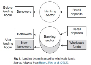
Hahm, Mishkin, et al. (2012) and Hahm, Shin, et al. (2012) note that the composition of bank liabilities provides valuable signals on lending booms, financial fragility and banking crises. In fact, large holdings of wholesale funds increase the willingness of the banking system to face greater risk exposure. Hence, the extent of wholesale liabilities could reflect the phase of the financial cycle and the degree of vulnerability to setbacks. Fig. 1 depicts the banking sector balance sheet before and after a credit boom. Clearly, this picture outlines the buildup of vulnerabilities associated with growth in wholesale funds.

Bearing in mind the previous discussion, the main objective of this paper is to study the empirical relationship between credit funding sources and the vulnerability of the Colombian banking system. From this crucial link, we propose a monitoring tool based on predictions of the probability of financial fragility. In particular, the empirical exercise estimates the probability of being in a situation of banking fragility as a function of the credit funding sources. The econometric exercises carry out a Bayesian averaging of logistic regression models that express a financial risk index in terms of retail deposits and wholesale funds. Our index aggregates four distinct risks: credit, profitability, solvency and liquidity. The estimations are performed using monthly Colombian data from the balance sheet for the entire banking sector and 12 individual banks between 1996 and 2013.

The results show the increasing use of wholesale funds, particularly to support credit expansion, entails potential elements of risk and, hence, episodes of banking fragility. Within them, foreign credit, interbank operations and securities redemption are relevant factors to identify most of such episodes. Therefore, monitoring credit funding sources becomes an essential tool in a macropru-dential scenario to prevent events of financial crisis.

The reminder of this paper is organized as follows. Section 2 presents the stylized facts of the dynamics of credit and its funding sources. Section 3 explains the construction of our measure of financial fragility, while Section 4 goes into the details of the econometric strategy. In Section 5, we perform the empirical exercises and present the results. Finally, Section 6 offers some conclusions.

2. Funding sources of banking loans

2.1. Accounting framework approach

We suggest financial fragility can be explained by credit funding sources. To illustrate this point, we adapt the Shin and Shin (2011) framework by starting with a simple accounting scheme traced from the balance sheet. Let us begin by defining the agents of the financial system as borrowers (domestic enterprises and households), creditors (households who offer retail deposits), banks (who channel resources from creditors to borrowers), and other creditors (additional local and external intermediaries), whose function is to provide funds (wholesale funds) to the local banking sector.

We adopt the assumptions that there exist n local banks (indexed by 1, 2, 3.....n), and that the domestic-household creditor sector is represented by n + 1. The other creditors sector (i.e. other domestic and external intermediaries) is indexed by (n + 2). Bank i has three types of assets: loans to final users (y_i), a portfolio in domestic securities (s_i), and loans to other creditors, who may be agencies within the banking sector itself and/or other intermediaries (local and foreign). The interbanking assets are noted by Σx_jπ_ji, where x_j represents the total debt of bank j and π_ji is the share of bank j's debt held by bank i. Notice therefore that π_j,n+1 is the share of the bank's liabilities held by the household-creditor sector (e.g. in the form of retail deposits), while π_j,n+2 is the share of the bank's liabilities held by other-creditors (e.g. in the form of wholesale funds). As long as the agents n + 1 and n + 2 do not use leverage, then x_n+1 = x_n+2 =0.

The balance sheet identity of bank i is given by

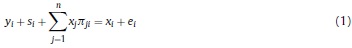
which means the total assets (left-hand side of (1)) are equal to debt (x_i) plus equity (e_i).¹

We can aggregate the set of banks and reorder the variables so that Eq. (1) can be expressed as

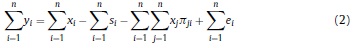
The resources in x_i can be broken down into retail deposits rd_i and wholesale liabilities wl_i. Eq. (2) is rewritten as

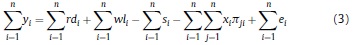
Considering the interbanking liabilities which are, implicitly, within the wholesale liabilities and the interbanking assets, both on the right side of Eq. (3), we can calculate the net interbanking operations as part of the wholesale funds (wf_i = wl_i - Σⁿ_j=1x_jπ_ji) so that Eq. (3) becomes

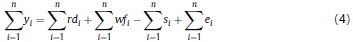
The left-hand side of (4) represents the total loans to final users granted by the banking system. The available funding sources are described on the right-hand side. Shin and Shin (2011) point out that financial fragility is associated with credit funding sources, and retail deposits are typically the most important ones. However, as mentioned previously, in periods of credit booms, that source is not enough to finance the bank's loans. Accordingly, banks seek to access to so-called wholesale funds from other types of agents (local and external intermediaries). Beyond recent literature has emphasized, we wish to call attention to another possible source of loan funding. It amounts to the redemption of investments in the case of banks that hold securities in their portfolios.

It should be noted that additional sources of loans funding could come from equity, particularly from the resources that exceeded the required reserve levels. We will show in the next section that banking risks could be exacerbated when loans (y) are increasing rapidly, thereby expanding banking vulnerability. Since y is highly correlated to risks, especially in credit booms, we will employ the right side of Eq. (4) to assess banking vulnerability.

2.2. Retail deposits and wholesale funds

We break down the total liabilities on the balance sheet into two groups of resources; namely, retail deposits and wholesale funds. In principle, retail deposits are the liabilities of a bank with non-bank domestic creditors. International evidence shows these funds are both the predominant source of banks' funding and the ones that grow in line with the aggregate wealth of households (Hahm, Shin, et al., 2012; Shin & Shin, 2011). The items contained within could follow the traditional criteria for classifications of monetary aggregates, which focus on the role of money as a medium of exchange. Therefore, retail funds include demand deposits, savings deposits, term deposits with different maturities, and small remaining deposits.

From a financial vulnerability perspective the distinction between retail and wholesale funding for banks is not captured sufficiently by the ease at which transactions are settled. Shin and Shin (2011) and Hahm, Shin, et al. (2012) recommend considering other classification criteria that deal with who holds the claims, particularly to properly understand the role of wholesale liabilities. The new approach implies to move toward a market-based financial system instead of deposit-based funding. For example, overnight repurchase agreements (repos) between financial institutions are a case of claims that are short-term and highly liquid, with very different systemic implications. In terms of liquidity, at the other extreme, there are long-term bonds issued by banks that are acquired (typically, but not exclusively) by institutional investors.

For Colombia, the wholesale funds will consist largely of bond emissions, institutional deposits from other intermediaries (e.g. deposits from second-tier banks), foreign credit, and interbank short-term liabilities (repos and other operations). Bond emissions are used normally to finance projects for the banks themselves, but also could eventually fund loans to third parties. Foreign credits correspond to resources for commercial credit, while interbank operations correspond to exceedingly short-term operations (intraday operations to cover liquidity shortfalls).

We use the balance sheet of the Colombian banking system, as provided by The Financial Service's Authority (Superintendencia Financiera), to analyze the banks' sources of funding. Specifically, our data set contains monthly information from December 1996 to March 2013 at two levels: the aggregate banking system and individual banks. We select a subset of 12 banks, while the total banking sector includes information on 25 banks. The 12 individual banks were selected due to availability of data for the entire sample period. Annex A summarizes the set of all credit funding sources, the definition of each one and its specific source, while Annex B reports the descriptive statistics of this set of variables.

Fig. 2 (left-side panel) shows the size and dynamics of retail deposits and the wholesale funds (as share of total liabilities) during the sample period. Retail deposits are the main source of credit funding (around 80%). In turn, the wholesale funds are the minority, more volatile and their share fluctuated between 10% and 20%. Concerning the composition of retail deposits, savings deposits still remain the preferred financial tool for households, followed by term and demand deposits (Fig. 2, right-side panel). Savings deposits account for half of the total, on average. Some degree of substitution between saving deposits and TDs (Term Deposits) is particularly evident as of 2002. So, while saving deposits were increasing, TDs became less attractive and vice versa. Panel B in Annex B also provides descriptive statistics on this set of covariates.

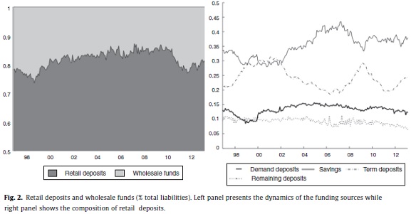
Fig. 3 (left-side panel) shows the dynamics of wholesale funds and their components during the sample period. Contrary to retail deposits, these funds exhibit high volatility and none of the components was dominant throughout the period. At the end of nineties, wholesale funds recorded the highest peak (just over 25% of total liabilities) and foreign loans were the most prominent. The leading role of foreign loans occurs before the Central Bank norm (Resolution 8 of 2000) that imposes restrictions on financial intermediaries in relation to foreign resources management. Subsequently, the wholesale funds are reduced gradually up to 15% by the mid-2000s. A new high peak in this fundings is observed between 2010 and 2012 (above 20% of total liabilities), but bonds and deposits from other intermediaries (deposits from second-tier banks) constituted the majority. The lowest share of foreign credit for the second part of the 2000s could be the result of several measures set by the Central Bank in 2007 to avoid the entry of foreign capital flows during a credit expansion period. In particular, the Central Bank employed the marginal reserve requirements, changing the rate from 0% to 27%. This measure was eliminated in 2008 in response to the international credit crunch.

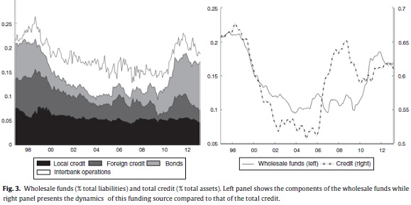
What is shown in the right-side panel of Fig. 3 is very interesting. It compares the dynamics of total credits granted by banks (as a percentage of total assets) to the dynamics of wholesale funds (as a percentage of total liabilities). The loans include credits to enterprises for commercial purposes; loans for household consumption; mortgages, and so-called microcredits, which are loans to very small firms. Both series seem to have a high positive correlation, at least up to 2006. Thereafter, the series diverge, perhaps because banks found other sources of funding.

2.3. Funding through securities

An alternative source of bank loan funding comes from the use of securities in the case of banks that hold important amounts of these assets. Why banks hold financial securities has to do with reasons that are beyond the scope of this paper. However, it is reasonable to think that, while it is typical for banks to re-balance their risks by granting loans at different maturities and across diverse activities, in practice, they also could do so by maintaining a significant portion of their assets in sovereign bonds, corporate shares and other securities, or simply could hold securities for profitability reasons. Nevertheless, what is remarkable here is the eventual redemption to fund growth in credit. Fig. 4 (left-side panel) shows the share of securities in bank assets, which is not stable and ranges from 10% of total assets at the end of the nineties to 35% by the middle of the next decade. Between January 2000 and July 2006, the value ofsecurities showed positive and negative changes which could be associated with policies to increase or liquidate holdings to fund bank loans and with revaluations due to price changes in the leader assets.

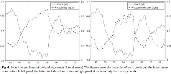
For a closer look at these issues, the right-side panel of Fig. 4 shows the dynamics of investment in sovereign bonds; namely, TES (the main securities bought by banks) versus total loans (both as share of total assets). We want to illustrate the clearly opposite trends of these two assets of the banking system, i.e. the banking system presumably uses resources from the sale of fixed-income investments to provide loans. Thus, while loans decreased progressively in the first part of the 2000s, the investments of banks in treasury securities increased. As we noted earlier, the trends change abruptly at the mid-2000s, when credit began to increase and, simultaneously, investments fell. There is no doubt the asset recomposition of banks registered in the second part of the 2000s was due to a change in strategic policy such that the redemption of sovereign securities could be used to fund new loans. The central bank report of March 2007 recognized these facts.²

International evidence indicating that commercial banks increasingly borrow wholesale funds to supplement traditional retail deposits has been also attributed to the competition for household savings from alternative investment agencies such as mutual funds, life insurance products, etc. (Huang & Ratnovski, 2010). Literature based on recent events in the United States and Europe also emphasizes that banks can use wholesale funds to expand lending, which could end up compromising credit quality (Agur, 2013). The hypothesis we explore in this paper is that wholesale funds can increase the fragility of banks, especially in phases of high credit expansion. However, an empirical evaluation first requires defining the concept of financial fragility.

3. Financial fragility

To characterize financial vulnerability empirically, we constructed a single indicator that collects most of the risks to which a bank is exposed. This indicator takes the form of a dummy variable and tries to identify periods in which a particular key risk, or some of them, generates an eventual warning situation for banks. As we will see in Section 4, this exercise is a crucial step in the development of our empirical strategy. The indicator is built for the total banking sector and for each individual bank.

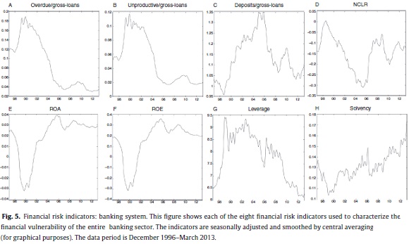
Four types of risk are taken into account: credit risk, liquidity risk, profitability risk and solvency risk.³ In turn, each is measured by two criteria: credit risk, by means of the ratios overdue/gross-loans and unproductive/gross-loans; and liquidity risk through the ratio of deposits to gross-loans and the non-covered liabilities ratio (NCLR). The third subset of profitability risk variables includes the return-on-assets (ROA) and return-on-equity (ROE) measures. The final set includes solvency and leverage risks, which capture the ability of an entity to meet its long-term commitments and to fund its projects, respectively. Annex A summarizes the definition of each risk and its specific source, while Annex B reports the descriptive statistics of this set of variables.

Regarding data, it should be noted that the banks in our sample have suffered from mergers and acquisitions, and the statistical format that captures the information on banks has changed as well (e.g. changing of definitions and variables). Therefore, we have made statistical adjustments to the original data so as to considerall these points and, hence, to make the time series consistent throughout the sample period.⁴ In addition, the original risk data exhibit numerous peaks in very short periods of time, which certainly generates noise. For this reason, the series were seasonally adjusted. Each of the financial risk indicators of the banking total system is plotted in Fig. 5.

To construct the financial fragility indicator, our technique starts by decomposing each risk into its trend and cyclical component using the Christiano and Fitzgerald filter (Christiano & Fitzgerald, 2001). This filter avoids the endpoint problem of the Hodrick and Prescott filter and is more flexible in handling windows for high frequency series. This approach allows us to identify both the highest and lowest phases of each variable. Periods of high cyclical component correspond to situations where exposure to a specific risk increased beyond its natural trend. We consider the highest peaks to be associated with periods of high risk exposure; hence, these periods entail phases of increased fragility.

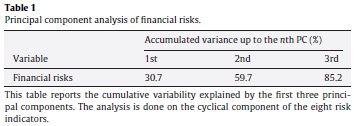
Decomposition of each risk leads to time series that reveal several periods of fragility. This is because each risk evaluates a different aspect of the health of banks. Accordingly, we use Principal Component Analysis (PCA) to find a common pattern among them. More precisely, we perform PCA on the cyclical component of the eight risks described above.⁵ The principal components are rotated using a Varimax rotation to obtain a better economic interpretation of our findings. Once we complete the rotation, we select the number of principal components (PCs) that will be used to construct our financial fragility dummy.⁶ Table 1 reports the accumulated variance up to the 3-PC, which jointly explains 85% of the total variance in the data and a large proportion of almost all the risks.

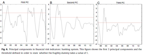
In the last step, we define banking fragility as those situations where the computed PC are above a threshold (Fig. 6), i.e. our dummy variable takes the value of 1 in those cases and 0 otherwise. The threshold is fixed (ad hoc) by using quantiles at 90% confidence for each PC. The first PC is an index that summarizes both credit and leverage risks. The second PC illustrates the influence of liquidity and solvency risks, while the third PC involves profitability risk. In order to check the robustness of this approach, we also compute our banking fragility dummy using alternative quantiles (95% and 85%). In doing so, we find no substantial differences in the results with both criteria.

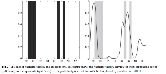
Left-Panel in Fig. 7 shows the periods of financial fragility for the total banking system (gray areas), while Right-Panel compares these areas with the probability of credit booms (Guarín et al., 2014). From the start of our sample (1996), we can distinguish three periods of relatively high financial fragility. The first one (2000-2002) is associated mainly with the downturn in the Colombian economy. The second period is related to the credit expansion in 2006-2007 and the capital restriction forced by the central bank. The third period (2009) is related to the fall in profitability in the sector, credit expansion in 2008 and, in some cases, liquidity problems. Following the ideas of Shin and Shin (2011), as mentioned, it is not surprising that periods of high financial fragility are associated with periods of credit expansion, as is evident in Panel B. The results at the individual bank level are shown later.

4. Model

We employ a Bayesian averaging of logistic regression models to estimate the probability that the banking system as a whole or a particular bank is in a position of financial fragility.⁷ Such a position is affected, in particular, by loan funding sources. We consider the following model:

where v_t = 1 if there is financial fragility at month t and v_t = 0 otherwise, α is the intercept, β is a R x 1 parameter vector, ε_t is the error term and X_TxR is the set of covariates that capture the different sources of credits funding. To capture some macroeconomic factor that affects financial vulnerability and that arises apart from the balance sheet, we include a leader indicator of economic activity as control variable z_t. Taking into account the variables of Eq. (4) in Section 2, we can rewrite (5) as where rd_t are the retail deposits, wf_t the wholesale funds (both as shares of total liabilities) and s_t the use of securities (as share of total credits).⁸,⁹

Let p(v_t = 1|θ; rd_t, wf_t, s_t,z_t) be the probability of being in a situation of financial fragility at time t, it can be defined as

where θ = [α'β'] and F is the cumulative logistic distribution function.

To deal simultaneously with both the model and the parameter uncertainty in our estimation, we run a BMA (Bayesian Model Averaging) estimation following Guarín et al. (2014) based on Raftery (1995) and Raftery, Madigan, and Hoeting (1997). The data set is denoted by D and = [M₁.....M_K] is the set of all models. So, M_K is the kth model considering a subset of the covariates which size is less or equal to R and θ^k its associated parameter vector.

Rewriting (7) in a BMA context, we get

where p(θ^k, M_k|D) is the joint posterior probability and the equation as a whole is a weighted average of probabilities in Eq. (7). Those weights are given by p(θ^k, M_k|D).

The reversible jump Markov chain Monte Carlo (RJMCMC) algorithm introduced by Green (1995) is used to estimate the BMA probability in Eq. (8) (see also Brooks, Friel, & King, 2003; Green & Hastie, 2009; Hoeting, Madigan, Raftery, & Volinsky, 1999 for additional details).

In order to compute a value of the BMA probability at which there is a clear signal of financial fragility problem we take a threshold value t∈ [0, 1] as the solution to the following minimization problem

where Φ(t) is the proportion of financial fragility's false alarms, γ(t) is the proportion of undetected fragility situations and Ῡ is the maximum value of y admitted by the policymaker.

The values of Φ(t) and γ(t) are calculated as proportions of the total number of observations in the sample. That is

where 1_{·}is a dummy variable equal to 1 if condition {·} is satisfied, and 0 otherwise. The variable _t(t) is defined as

Note that for a given probability p(ν_t = 1|θ^k, M_k; D), the number of estimated periods of financial fragility depends on the threshold T. If the latter is very small, then we will have many situations of financial fragility that could be false alarms. On the contrary, if t is very large, then we will have few warnings and the probability of having undetected periods of financial fragility would be greater.

5. Results

Certain technical details should be highlighted before presenting the results. The probabilities of being in a situation of financial fragility at time t are estimated on the set of computed data [ν_t, x_t], and the dependent variable v_t corresponds to the indicator estimated in Section 3. The set of regressors x_it includes both contemporary covariates and up to six (6) lags of each one. The BMA estimates are performed by means of a Markov chain with 220,000 draws where the first 20,000 draws are burned-up to avoid the noise in the choice of the initial seed. We use a Reversible Jump Markov Chain Monte Carlo method to simulate the draws, and the draw chains were constructed using the Metropolis-Hastings algorithm. We assume the prior model probability is p(Mk) = 1/K, for all k = 1.....K, and the prior distribution of θ^k is N(0^k, 10 -I^k) where the zero vector 0^k and the identity matrix I^k change their size with the model M_k. The threshold probability t is computed by solving the minimization problem (9) with a maximum value of undetected fragility periods Ῡ equal to 5% of observations in our sample.

The sample includes monthly data from December 1996 to March 2013. All estimations are performed for either the total banking sector or individual banks. At the end of this section, we also present empirical results for the logit panel data model with fixed effects, using an adapted version of Eq. (7).

5.1. Total banking sector

In the first exercise we compute the logistic regression model (7) for the total banking sector. The BMA parameters are used to estimate the probabilities of being in a situation of financial fragility. Fig. 8 illustrates the results. The solid line displayed between 1996 and 2013 shows the estimated values of the probability, the gray areas correspond to periods of financial fragility previously identified via the risks indicators, and the dashed line defines the threshold, which is estimated at 33%. With the latter percentage, the probability of detecting a period of financial fragility is 88%, while the probability of having no false alarms is 82%.

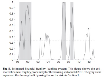
The results exhibit an excellent fit between the estimated probability and the identified periods of financial fragility, and the adjustment is generally quite fast. This means probability takes high values when there are periods of financial vulnerability, while it is close to zero when there is no fragility. The BMA probability, which depends on the resources for bank funding, identifies seven episodes of financial fragility. What is very interesting is that three of them are not captured by the risk-based dummy variable: at the middle of 2003, in 2004 and, with a higher probability value at the end of 2011. These findings are very important, because they suggest that during these three periods, the banking system exhibited a significant degree of vulnerability through its funding sources, but these situations were not captured by the standard risks. Based on these outcomes, monitoring the sources of bank funding could be a complementary tool to assess their state of fragility. This suggestion is the main policy implication provided by this paper.

The estimated probability highlights two episodes of financial fragility at the end of the 1990s. The first takes place in the second half of 1998 and at the beginning of 1999. Not surprisingly, these events coincide with the credit boom identified by Guarín et al. (2014). After that, the probability declines to less than 20%. Subsequently, there is a rise in probability to very high values, showing new episodes of vulnerability; namely, in the second half of 1999 and the last quarter of 2000. These two episodes are captured by the dummy variable. As mentioned, these episodes are associated with one of the worst downturns in the Colombian economy, which ultimately led to a financial crisis.

In the first half of the 2000s, the BMA probability finds a new set of episodes of financial fragility. However, they are not captured by the risk-based dummy variable. The first features a peak in the third quarter of 2002, which might be associated with the increase in market risk due to liquidity problems in the public debt market. The second peak reflects an increase in financial fragility between the second-half of 2003 and the first-half of 2004, which seems to be linked to a large expansion in credit. A look at wholesale funds in detail shows both episodes are clearly dominated by interbanking operations. In the first one, foreign resources also play an important role as a result of the process of catching-up after the recession and the high values achieved by the foreign exchange rate.

Between mid-2006 and mid-2007, a new financial fragility episode (the fifth one) is captured by our probability. This period is characterized by a strong expansion in credit and entries of capital flows. The Colombian central bank was forced to take measures to avoid a possible credit boom. The central bank increased the levels of the marginal legal banking reserve to deal with the perverse effects of these capital flows. The next episode of financial fragility occurs in the second half of 2008. It is closely related to the collateral effects of the international financial crisis, which also had an impact on the Latin American economies. Concerning the final years, we found the probability features a period of fragility between the second half of 2011 and the first quarter of 2012. Once again, the risk-based dummy variable is not able to capture this episode, which is associated mainly with a strong expansion in credit, coupled with capital inflows and high asset prices. Not surprisingly, foreign resources are the main wholesale funds that explain the higher probability.

Table 2 reports the posterior inclusion probability (PIP), the posterior mean, the posterior standard deviation, and the sign certainty, for all variables selected by BMA methodology as determinants of probability.¹⁰ We denote the contemporary value and the i lags of the variable (·) as L_i. The table shows the statistics for the 20 covariates with the highest PIP values of the model. According to the criterion, the most important variables in the estimation are Foreign Credit (L1), Economic Activity Index (L5), Interbank Operations (L4, L6, L5), Securities redemption (L4, L2, L1) and Bond issuance (L0).

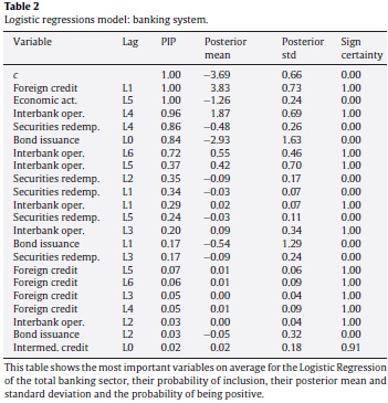
The increase in the credit funding sources such as foreign credit, interbank operations and credit from other domestic intermediaries, all of them being an important part of wholesale funds, has a positive effect on the probability of financial fragility, as expected. On the contrary, an increase in the use of securities, bond issuance, and a rise of economic activity, has a negative impact on the probability. The use of securities has the expected sign (see Eq. (6)) confirming the hypothesis that the banking system uses resources from the sale of fixed-income investments to fund loans.

Regarding the other two variables, we think that, for instance, in the middle of downturns, the income of households is negatively affected and borrowers have difficulty in paying their debts, thereby increasing the vulnerability of the banking sector. This effect has a lag of six (6) months, while income is reduced and they start to abandon their obligations. We also presume that bond issuance could reflect the health of financial entities; i.e. banks could issue bonds particularly when they are looking for funding to operate new projects instead of issuing bonds to fund new loans. Finally, we note that retail deposits do not appear as a determinant of the BMA probability, as expected. The above is because in periods of loan expansion (and fragility), these funds are not enough to cover the demand for bank lending, as remarked by literature. Consequently, banks make use of wholesale funds rather than traditional or retail deposits.

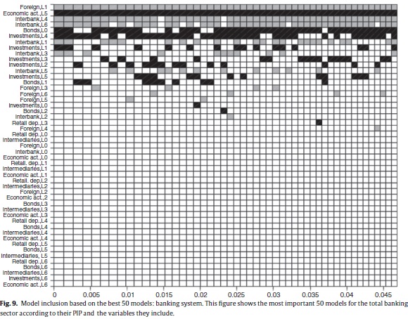
Fig. 9 illustrates how important the variables in the 50 "best" models are, according to the highest associated model probabilities. The models are shown on the horizontal axis, ordered by importance, and the covariates on the vertical-axis, ordered by their PIP. The colored boxes show the variables included in each model and their sign. A gray color represents a positive variable while black, a negative one. The model with the highest probability includes nine (9) covariates: foreign credit (L1) and interbank operations (L4, L6, L1, L3) entering with a positive sign, and bond issuance (L0), economic activity (L5), and securities (L4, L2, L1, L5) entering with negative sign. In addition, the variables seem to keep their signs throughout the models where they are included. Moreover, the graph shows the idea of convergence in the BMA technique, where the first models consider the possibility of using a lot of variables, while the last models take only the most important ones.

5.1.1. Predicting financial fragility episodes

The models computed in previous sections can be useful to predict the short term probability of being in an episode of financial fragility at time t + h, based only on credit funding information up to time t. Note that h stands for the time horizon of our direct forecast. This exercise provides a valuable tool for monitoring the short-term health of individual banks and the aggregate system in order to prevent possible episodes of financial instability.

Specifically, we carry out the BMA estimation of the probability P^BMA(ν_t+h = 1|D) for t = 1.....T and h = 1.....6.

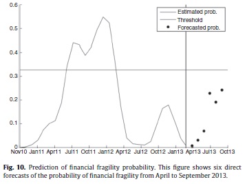
Fig. 10 plots both the in-sample estimate of the probability of financial fragility for h = 0 (i.e. solid line in Fig. 8) and the results of our prediction for h = 1.....6 (black points). As mentioned above, each point represent the direct forecast of the probability at time T + h, given the data on credit funding sources up to time T = March of 2013, which is our last available date in the sample. For instance, with h = 6, we predict the probability of being in a fragility episode for September of 2013 (about 0.25). Fig. 10 shows our entire set of predicted probabilities is below the estimated threshold for all time horizons; hence, there are not signals of banking instability in the short-term.

5.2. Individual banks

The probability estimation for financial fragility at the individual bank level uses a sample of 12 entities. With this exercise, we try to assess the effects of the funding strategy of each bank on its financial fragility. The procedure also allows us to enhance the performance of our model in terms of the estimation. In addition, the individual fragility assessment becomes a useful tool for monitoring. Once again, all the BMA probabilities are estimated on the set of data [x_{i t}, ν_{i t}], where the dummy variable of financial fragility was constructed for each bank following the description in Section 3.

We cluster our sample of financial institutions in two groups: The first group includes four large banks and the second one includes eight medium and small-size banks. The classification is based on their share of total assets. The large-size bank group accounts for 42.7% of the total assets of the banking system, while the medium- and small-size group account for 23.5%. This characterization allows us to analyze in detail the dynamics of financial fragility and its relationship to credit funding sources between similar sized banks, in order to reduce the high heterogeneity between them. Although the estimation is at an individual level, we want to generalize the conclusions at the group level.

Figs. 11-13 show the results of our individual estimation. For each bank, we plot (left column) the estimated BMA probability of financial fragility (solid-line). This probability is compared to the risk indicator, which represents the periods of financial fragility as described in Section (3). We also plot the threshold (dash line) computed for each bank. Each panel includes a table (right column) with the BMA results: PIP, posterior mean, posterior standard deviation and sign certainty for the eight most important variables.

5.2.1. Large-size banks

Fig. 11 shows thatourmethod is able to capture the main periods of financial fragility for large-size banks, as identified through the risk-based dummy variable. The fit of our model, with respect to the periods of banking instability, is quite successful. Three of the four banks in the group have a threshold at around 22% and their probability of having no false alarms is equal to 77%. In particular, bank 3 has a very good fit, which leads to a higher threshold of 48%, and better probability indicators. In fact, for this specific bank, the probability of detecting a period of financial fragility is 99%.

In general, the episodes of financial fragility for this group of banks are in line with those found for the total banking sector: financial fragility at the end of the 1990s, between the fourth quarter of 2006 and the first half of 2007, and in the second-half of 2008. Unlike the estimated results for our total banking sector, we are unable to detect for all banks, at an individual level, the financial fragility in the third-quarter of 2002 and the episode between the second-half of 2003 and first-quarter of 2004. The results also show the large-size banks experienced an episode of vulnerability in the second-half of 2011 and first-half of 2012, which is in good agreement with the results for the total banking sector.

We also find economic activity is an important covariate, according to their PIP. In three of four banks, this variable has a PIP near 100%. This result suggests fragility for this group of banks is related directly to changes in economic activity; i.e. they are more vulnerable during recession periods, as expected. There are other covariates with an impact on the probability of fragility (e.g. foreign credit, investments substitution and interbank operations). In particular, banks 1,3 and 4 are very similar in terms of the explanatory covariates of the financial vulnerability, while bank 2 differs. For that bank, movements in foreign credit lead the dynamics ofits probability of financial fragility.

5.2.2. Medium and small-size banks

Figs. 12 and 13 show the estimation results for medium and small-size banks, respectively. These results are quite similar compared to one another. Even though episodes of financial fragility measured by risks are not uniform throughout the banks, in general, they are captured appropriately by BMA probability. However, the number of episodes computed by the probability for these groups of banks is distinct from those found for the aggregate banking system and even for large-size banks. For the medium-size banks, for instance, episodes of financial fragility are more disperse over time and shorter. In the case of small-size banks, there are more areas highlighted as periods of instability, but their duration is also shorter than those for the total sector.

Although our model has a lower fit in these cases, the exercises are able to capture the periods of financial fragility highlighted by the gray areas computed in Section 3. With the exception of Bank 6, the most important covariates to explain the instability of medium-size banks are interbank operations, foreign credit, and securities redemption. For this group, the threshold is 15%, on average, and the probability of detecting financial fragility periods is reduced to 62%. The emission of bonds is another important covariate within the analysis. As mentioned earlier, we assume this variable could provide signals of good health and using the resources obtained through bonds to expand the business instead of financing credit. We also highlight, within the analysis, that economic activity is no longer a decisive variable for estimating the probability of financial fragility. The PIP of all the variables is lower than the ones of large-size banks. These results indicate that variables are not completely decisive in the determination of the probability. For Bank 6, specifically, our model does not provide a good fit and the results are not conclusive.

In the case of the small-size banks, the threshold probability is 19%, on average, and the probability of having no false alarms is 74%. Hence, the probability of detecting financial fragility periods is 66%. The model is able to capture the financial fragility periods at the end of the 90s, as well as the ones registered in 2008 and 2009. In some cases, we found new episodes in 2006 and 2007. We also point out financial fragility periods at the end of 2011 and in the first-quarter of 2012, when consumer credit grew very quickly. In the particular case of Bank 11, the fit of the model is not good enough.

The results for small banks also show that the most important variables, according to their PIP, are securities redemptions, interbank operations and foreign credit. In most cases, the covariates with high lags (L5, L6) are more relevant. In particular, we suggest that covariates with those lags are providing signals for the determination of financial fragility in the long run. In other words, variables are giving signals about how changes in the cyclical component of a particular variable today, as interbank operations or foreign credit are indicative of a future variation in the financial fragility.

5.3. Panel data with fixed effects

To take into account the individual characteristics ofthe full set of banks in our sample, we run a logistic regression model with panel data and fixed effects adapting Eq. (7). Fig. C.1 in Annex C shows the results of the estimation. Each panel in this figure presents the estimated BMA probability for one bank compared to its own financial fragility areas (based on risks). Once again, the estimated probability is denoted as a thin solid line and the threshold probability is plotted as a dash line.

In general, we see the estimated probability of financial fragility coming from funding sources does not have a good fit with respect to the predefined episodes based on risks. Given the low fit, the computed threshold probability is set at 17% to keep a maximum tolerance of 5% of undetected episodes of fragility. In addition, we found a very low probability of having no false alarms.

We must bear in mind that episodes of fragility identified specially for medium and small banks are a bit different from those identified for the total sector. Moreover, credit funding sources also have distinct dynamics among banks. In fact, the results of our exercise with panel data and fixed effects show the heterogeneity among banks is too high, and trying to summarize their individual characteristics in a set of particular covariates with a good fit of the data is a difficult task. Hence, the high heterogeneity found in the data for individual banks with respect to financial fragility areas and credit funding sources led us to use the approach based on the estimation of individual logistic regression models for each bank.

6. Conclusions

The Colombian banking sector is relatively small, not quite open internationally, and is in a process of deepening. Currently, total banking assets are over one-third of GDP (40%), which is the average for Latin American emerging economies. The increasing use of wholesale funding to support bank loans, particularly for some phases of credit expansion, could be a new characteristic of the banking system. This feature, in turn, probably means a greater financial fragility during these periods, which needs to be monitored carefully in the interest of having a sound financial system.

The previous conclusions arise from this paper, which provides empirical support on the relationship between the funding sources of credit and the financial fragility of the Colombian banking system. In particular, we were interested in exploring how the increasing use of wholesale funding to support bank loans, especially in credit expansion phases, is a potential source of financial instability. Among the wholesale accounts with greater impact we identify foreign credits, interbank short-term operations and bond issuance.

Regarding methodological details, our data set contains monthly balance sheets from December 1996 to March 2013 at both levels: the aggregated banking system and individual entities (12 banks which account 65% of total banking assets). Our empirical strategy first implied defining a statistical model to measure the financial fragility via the standard risks indicator and, subsequently, to carry out the logistic time series and panel data regressions, based on Bayesian technique, to estimate and predict the probability of episodes of banking fragility based on loan funding sources. In the first step we employed an ample set of indicators to capture the main four risk categories: credit risk, liquidity risk, profitability risk and solvency risk.

Our model identifies seven episodes of financial fragility since 1996. What is truly a novel result is that three of them are not captured by the standard risk indicators, i.e. there were three episodes during which the banking system exhibited a significant degree of vulnerability on the basis of its funding sources, but these situations were not captured by the standard risks indicators. Consequently, changes in funds used for lending could be a potential source of financial instability, and monitoring them could be a complementary tool to assess their state of fragility. This suggestion is highly important for policymakers and greatly relevant for policy discussions on regulation of financial institutions. Even though the exercise is performed for the Colombian banking system, it could serve as reference to be applied to other emerging economies.

Finally, the findings noted in this paper seem to be in line with a burgeoning amount of recent literature that associates both credit cycles and financial stability with the dynamics of bank lending. According to this literature, traditional retail deposits are not enough to cover the demand for lending during phases of credit expansion; hence, banks access wholesale funds as alternative funding sources. We call attention to the fact that, apart from the Korean case, the empirical analysis on this subject in emerging economies has been limited.

Conflicts of interest

The authors have no conflicts of interest to declare.

Pie de página

¹ Note that for i = j, the interbank assets are equal to zero.

² Indeed, the BR (Banco de la República)-March-2007 report said that "... the credit establishments restored their assets in favor of the loans ... so the share of loans in total assets increased from 50% to 58% between December of2005 and 2006, while the share of investments (of which public debt securities represent a 62%) was reduced from 32% to 24%..." [Original report written in Spanish].

³ Unfortunately, by restrictions on the data, there was not possible to estimate market risk at individual bank level, and hence, for the sake of consistency we did not use this indicator at the aggregated level. Nevertheless, other financial risks capture indirectly the exposition and perceptions ofmarket risk.

⁴ We made two major changes: first, series were adjusted by taking into account an amendment in the Accounts Plan (Plan Unico de Cuentas) since 2002. Second, we took as reference an internal document from Banco de la República (the Central Bank) for the chronological history of mergers and acquisitions between banks.

⁵ Note that we run the PCA on the cyclical component of the time series and not viceversa. This is because our original series are not stationary, and therefore, a PCA on those series could be wrong. Hence, first, we compute the cyclical component, which is stationary for each time serie, and then running the PCA.

⁶ In general, our banking fragility dummy in all our empirical exercises considers two or three PCs that capture around 80% and 90% of the data variance.

⁷ This technique is used by Guarín et al. (2014) to estimate a probability of having a credit boom in Latin American emerging economies.

⁸ We also use the variables rd and wf as a proportion of M2. Although the results are not shown, these do not change significantly.

⁹ We left out variable (e_i) of Eq. (4) as a source of funding because its inclusion (defined as both total equity and equity that exceeds legal reserves) generates statistical problems that lead to overfitting. In the case where we restricted its sign to be positive as expected, it makes the exercise to lose signs robustness of the other variables.

¹⁰ The PIP stands for the probability that an explanatory variable is included in the model. The sign certainty presents the probability that the estimated coefficient is positive.

References

Agur, I. (2013). Wholesale bank funding, capital requirements and credit rationing. Journal of Financial Stability, 9(1), 38-45.         [ Links ]

Bordo, M., & Haubrich, J. (2010). Creditcrises, moneyandcontractions: Anhistorical view. Journal of Monetary Economics, 57,1-18.         [ Links ]

Borio, C. (2012). The financial cycle and macroeconomics: What have we learnt? In B1S Working Paper 395, Bank for International Settlements.         [ Links ]

Brooks, S., Friel, N., & King, R. (2003). Classical model selection via simulated annealing. Journal of the Royal Statistical Society, 65(2), 503-520.         [ Links ]

Bruno, V., & Shin, H. (2013). Capital flows and the risk-taking channel of monetary policy. In NBER Working Paper 18942.         [ Links ]

Cerra, V., & Saxena, C. (2008). Growth dynamics: The myth of economic recovery. American Economic Review, 98(1), 439-457.         [ Links ]

Christiano, L., & Fitzgerald, T. (2001). The band pass filter. In NBER Working Paper 7257.         [ Links ]

Claessens, S., Kose, M., & Terrones, M. (2012). How do business and financial cycles interact? Journal of International Economics, 87, 178-190.         [ Links ]

Damar, H., Meh, C., & Terajima, Y. (2010). Leverage, balance sheet size and wholesale funding. In Bank of Canada Working Paper 39.         [ Links ]

Drehmann, M., Borio, C., & Tsatsaronis, K. (2012). Characterising the financial cycle: Don't lose sight of the medium term. In B1S Working Paper 380, Bank for International Settlements.         [ Links ]

Frankel, J., & Saravelos, G. (2010). Are leading indicators of financial crises useful for assessing country vulnerability? Evidence from the 2008-2009 global crisis. In Technical report, NBER Working Paper 16047.         [ Links ]

Goldstein, M., Kaminsky, G., & Reinhart, C. (2000). Assessing financial vulnerability, an early warning system for emerging markets: Introduction.         [ Links ]

Gourinchas, P., Valdes, R., & Landerretche, O. (2001). Lending booms: Latin America and the world. In NBER Working Paper 8249.         [ Links ]

Green, P. (1995). Reversible jump Markov chain Monte Carlo computation and Bayesian model determination. Biometrika, 82(4), 711-732.         [ Links ]

Green, P., & Hastie, D. (2009). Reversible jump MCMC. In University of Helsinki Working Paper 155.         [ Links ]

Greenwood, R., Landier, A., & Thesmar, D. (2012). Vulnerable banks. In NBER Working Paper 18537.         [ Links ]

Guarín, A., González, A., Skandalis, D., & Sánchez, D. (2014). An early warning model for predicting credit booms using macroeconomic aggregates. Ensayos Sobre Política Económica, 32(73), 77-86.         [ Links ]

Hahm, J., Mishkin, F., Shin, H., & Shin, K. (2012). Macroprudential policies in open emerging economies. In NBER Working Papers 17780, National Bureau of Economic Research.         [ Links ]

Hahm, J., Shin, H., & Shin, K. (2012). Non-core bank liabilities and financial vulnerability. In NBER Working Paper 18428, National Bureau of Economic Research.         [ Links ]

Hamann, F., Hernández, R., Silva, L., & Tenjo, F. (2014). Leverage pro-cyclicality and bank balance sheet in Colombia. Ensayos Sobre Política Económica, 32(73), 50-76.         [ Links ]

Hoeting, J., Madigan, D., Raftery, A., & Volinsky, C. (1999). Bayesian model averaging: A tutorial. Statistical Science, 14(4), 382-417.         [ Links ]

Huang, R., & Ratnovski, L. (2010). The dark side of bank wholesale funding. Journal of Financial 1ntermediation, 20(2), 248-263.         [ Links ]

Hume, M., & Sentance, A. (2009). The global credit boom: Challenges for macroeconomics and policy. Journal of 1nternational Money and Finance, 28(8), 1426-1461.         [ Links ]

Jorda, O., Schularick, M., & Taylor, A. (2012). When credit bites back: Leverage, business cycles, and crises. NBER Working Paper 17621.         [ Links ]

Mendoza, E., & Terrones, M. (2008). An anatomy of credit booms: Evidence from macro aggregates and micro data. In NBER Working Paper 14049.         [ Links ]

Raftery, A. (1995). Bayesian model selection in social research. Sociological Methodology, 25, 111-164.         [ Links ]

Raftery, A., Madigan, D., & Hoeting, J. (1997). Bayesian model averaging for linear regression models. Journal of the American Statistical Association, 92(437), 179-191.         [ Links ]

Reinhart, C., & Reinhart, V. (2010). Afterthe fall. In NBER Working Paper 16334.         [ Links ]

Schularick, M., & Taylor, A. (2012). Credit booms gone bust: Monetary policy, leverage cycles and financial crises, 1870-2008. In NBER Working Paper 15512.         [ Links ]

Shin, H., & Shin, K. (2011). Procyclicality and monetary aggregates. In NBER Working Paper 16836.         [ Links ]

Annex A.

Annex B.

Annex C.