


 English (pdf)
 Article in xml format
 Article references
 Send this article by e-mail
 Cited by SciELO
  Cited by Google
  Similars in
SciELO
Similars in
SciELO  Similars in Google
 Permalink
How do capital requirements affect bank behavior along the business cycle? Are capital requirements capable of delivering a more stable macroeconomic environment in the face of shocks? General interest on these questions has increased since the onset of the recent financial crisis, and particularly since the Basel Committee on Banking Supervision (BCBS) gave a prominent role to macroprudential policy tools in the principles established in the regulatory framework widely known as Basel III.
Empirical literature on the effects of macroprudential policy and its interaction with the business cycle has been limited due to the small number of countries that have adopted any form of macro-prudential tool and to the yet relatively short experience with their use. Considering dynamic provisioning and countercyclical capital buffers (two widely discussed tools highlighted by Basel III), 119 countries have adopted either of them (all of them after 2005), and only two have introduced both. Up to this point, good sources of exogenous variation are relatively scarce, making it difficult to establish a successful empirical identification strategy. As a result, theoretical models offer more fertile grounds for obtaining insights into the functioning and effects of macroprudential policy tools.
This paper attempts to tackle those questions by building an equilibrium model of the macroeconomy that incorporates a bank, financial frictions, default and capital requirements. The model incorporates the decisions of patient and impatient households who make choices on optimal levels of consumption, work and enjoyment of housing services. Households also decide how much to save or borrow for the sake of consumption (consumer credit borrowing) or the provision of housing services (mortgage credit borrowing). Borrowing for either purpose is subject to credit constraints: the amount borrowed is constrained by the expected value of labour income or the stock of housing services. The model also includes intermediate and final goods producers; it is assumed that the former must borrow in order to finance working capital requirements (business or commercial credit borrowing). Saving and borrowing is intermediated by a bank facing capital requirements that differ for each of the three credit categories (consumer, mortgage, business). In addition, each type of borrowing has a different probability of default which depends on aggregate conditions. Finally, the model includes a Central Bank/Regulator who sets the interest rate on deposits and exogenously decides on capital requirements.
Contrasting with earlier work on equilibrium models with financial frictions, this paper employs a penalty function following Den Haan and De Wind (2012) in order to model minimum capital requirements. More specifically, the model introduces a cost to the bank which depends on the distance between observed and required capital. The parameters of the penalty function are chosen so that this cost becomes prohibitively high as observed capital converges from the right to the minimum, and is negligible otherwise. Compared to occasionally binding leverage constraints, this specification is easier and quicker to compute and it is flexible enough to allow for changes to the specific form of macroprudential policy/capital requirements. As such, it offers a promising strategy to deal with this type of constraints in equilibrium models. In addition, taking into account the wide variation in business cycle properties across different credit categories, the model introduces a non-trivial choice of credit composition for the bank. Total credit in the model corresponds to the aggregation of consumer, business and mortgage loans. The choice of loan supply for each of these credit segments takes into account their individual interest rates and their (endogenous) default rates. Loan supply will also depend on the regulatory requirements of each credit segment in terms of bank capital.
The paper focuses on the examination of the impulse-response functions of the model to study how the equilibrium relationship between the real economy and the financial system (the bank) changes in response to shocks. By comparing the response of the economy with or without capital requirements (that is, with or without the penalty function) it is also possible to discern whether this policy instrument contributes to deliver a smoother response of the economy to different shocks. The paper will specifically focus on the effect of capital requirements on the composition of bank funding as a main driver of the response of the economy to shocks. Given that risk (probability of default) is orthogonal to the choices of the bank, the model does not feature the standard, risk-taking channel studied elsewhere in the literature. In addition, given that the bank knows in advance which fraction of loans will be repaid (and plans its funding structure accordingly), macroeconomic or financial shocks in the model do not destroy the left-hand side of the balance sheet of the bank, and therefore do not deplete capital as in the well-known bank capital transmission channel of monetary policy (see Van den Heuvel (2006)). Thus, the model does not feature the standard leverage constraints channel of amplification of capital requirements studied elsewhere either. In the model, the main effect of capital requirements in the model is to disrupt the ability of the bank to change the composition of its funding sources. In the absence of capital requirements, any shock that reduces the deposit rate will incentivize the bank to switch away from bank capital into deposits, thus increasing the demand for deposits and dampening the effect of the shock on interest rates and the price of housing services. The main effect of capital requirements in the model is to disrupt the ability of the bank of switching to cheaper funding sources (deposits) after a shock. Capital requirements thus have the effect of amplifying the response of aggregate variables to shocks through the composition of the right-hand side of the balance-sheet of the bank (a channel that might be described as the bank funding composition channel).
Besides contributing to the understanding of the effects of capital requirements through this bank funding composition channel, the model also provides a framework for the quantitative analysis of the propagation of financial shocks in an emerging economy. The model is therefore useful to construct consistent scenarios after a shock which include the endogenous feedback effects between the real and the financial sectors of the economy. This is useful for stress testing exercises carried out by central banks and regulators which generally require some form of macroeconomic scenario as a starting point which ideally should include those feedback effects in a consistent fashion.
1. Related literature
This paper builds on insights from two strands of the literature that have been thus far developed separately. Firstly, at least since Matsuyama (2008) there has been an active area of research on the implications of credit composition both for economic growth and the business cycle. According to Matsuyama (2008), the particular properties of the development process, and the volatility of the business cycle depended on the composition of credit between categories that differ on pledgeability or collateralizability. Closer to the work in this paper, Saade, Osorio, and Estrada (2007) extend the model by Goodhart, Sunirand, and Tso-mocos (2006) to study the problem of financial stability in a general equilibrium framework with banks and default where there are different loan categories (consumer, mortgage and business) subject to different capital requirements and with different reduced form specifications for loan demand. They conclude that financial fragility is closely related to the equilibrium composition of banks’ loan portfolio. From an empirical point of view, Haan, Sumner, and Yamashiro (2009) illustrate the differing responses that different credit categories (mortgage, business) exhibit after a monetary policy shock in Canada. They conclude that the composition of credit is therefore crucial to understand the transmission mechanisms of monetary policy. Finally, Aghion, Angeletos, Banerjee, and Manova (2010) study the effects of the composition of investment (and credit) between short-term and long-term projects, to conclude that long-lasting recessions can be explained by the switch from long-term to short-term credit after financial shocks.
This paper also follows recent work on the implications of finance in dynamic, stochastic, general equilibrium models of the macroeconomy. Models in this field generally include heterogeneous agents and financial frictions (important references at this respect include Brunnermeier and Sannikov (2014) and Gertler and Kiyotaki (2010)); more recently, work has been expanded to study the role of macroprudential policies in preventing episodes of financial stability. The model in this paper is closest to Gambacorta and Karmakar (2016) and is based on the work by Agenor, Alper, and da Silva (2013), Gerali, Neri, Sessa, and Signoretti (2010) and Agenor and Zilberman (2015). Importantly, we borrow from Agenor et al. (2013) the strategy to model bank capital accumulation as the problem of choosing an optimal capital buffer taking into account both capital requirements and capital adjustment costs, and the idea of capturing equilibrium default rates using reduced forms. It is on top of this model structure that we include several loan categories with different capital requirements and a richer structure for the probabilities of default of these categories. The welfare implications of different macroprudential policy rules in the context of general equilibrium models are studied by Nogueira and Nakane (2015), and the specific effects of dynamic provisioning on the prociclicality of the financial system is explored by Agenor and Zilberman (2015). An important aspect not considered in this paper is the welfare effects of the coordination between monetary and macroprudential policies studied by Angelini, Neri, and Panetta (2014). One crucial element of the model in this paper is the effect of capital requirements on loan supply and bank behaviour. Capital requirements have effects on equilibrium interest rates, on the composition of the loan portfolio and on the propagation of shocks. Our paper therefore also builds on the findings by Meh and Moran (2010) regarding the importance of bank capitalization to understand the transmission of shocks across the macroeconomy.
This paper unfolds as follows. Section 2 studies the main stylized facts about the financial cycle in the Colombian economy. Section 3 presents the structure of the model. Sections 4 and 5 together consider the performance of the model under different types of macro-shocks. Finally, Section 6 offers some reflections as concluding comments.
2. Motivation: credit composition and the business cycle
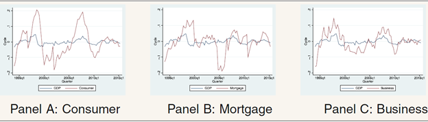
The importance of allowing for different credit categories (and for a non-trivial choice problem for banks as to the composition of their loan supply) is highlighted by the remarkable differences in the cyclical behaviour of consumer, business and mortgage credit and their rates of default. Table 1 presents the cyclical component of real GDP and the real stock of consumer (Panel A), mortgage (Panel B) and business credit (Panel C) in Colombia for the period between 1994 and 2015. All three credit categories are procyclical: the crash of the Colombian economy in 1999-2000 is reflected in steep falls of the cyclical component of credit. Credit also falls below trend during 2009-2010, a period which is associated with the financial crisis in developed economies.
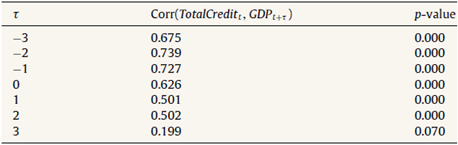
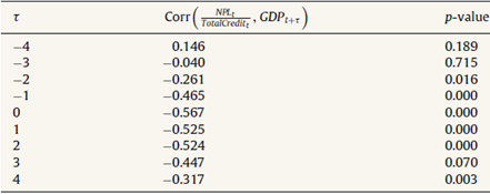
The contemporaneous prociclicality of all credit categories is also indicated by the correlation between the cyclical component of real GDP and total credit in Table 2, calculated using data from the same time window. The correlation is positive and statistically significant at three lags and leads. Table 3 indicates the correlation between the cyclical component of real GDP and the ratio of non-performing loans (NPL) to total credit, a measure of credit quality. Interestingly, although this correlation is negative and statistically significant at most lags, there is a positive correlation (although not statistically different from zero) between real GDP and NPL four quarters ahead. This may be an indication of relaxing credit standards during economic booms that end up reducing the quality of total credit afterwards.
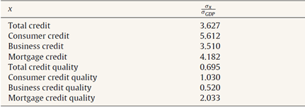
The cyclical behavior of aggregate credit tends to hide wide variation among credit categories. Table 4 presents the relative (to GDP's) standard deviation of the cyclical component of consumer, business, mortgage and total credit, and credit quality (measured as described above) for each of the same categories. Total credit is observed to be more than three times as volatile as GDP, whereas total credit quality is somewhat smoother (its standard deviation is 69% that of GDP). Interestingly, of all credit categories, consumer credit seems to be the most volatile (5.6 times as volatile as GDP), followed by business credit. This is interesting so long as most business cycle research has found consumption to be one of the least volatile macroeconomic aggregates. At the other end of the spectrum, mortgage loans turn out to be the least volatile, again in contrast to residential investment, which is normally found to be more volatile than consumption. Possibly due to the difficult conditions faced by mortgage borrowers during the period of analysis, mortgage credit quality is twice as volatile as GDP, whereas consumer credit quality has the same standard deviation, and commercial credit is half as volatile.
In summary, the aggregate behavior of total credit at business cycle frequencies, although intuitive, masks wide variation in the cyclical component of subcategories of credit. This observation motivates the adoption of a model which is capable to include several credit types that differ in key respects. In particular, the model interprets differences in the cyclical behavior of mortgage, consumer or commercial credit as arising from different degrees of financial frictions, different borrower preferences or variation in the volatility of shocks to which different credit categories are exposed. It is against the backdrop of these stylized facts on credit categories that the model presented below is motivated.
3. The model
The model is based on previous work by Gerali et al. (2010) and Agenor et al. (2013). The economy is composed by ex-ante het-erogenous households which differ in their discount factor. The discount factor for patient households, βp, is higher than that of impatient households, βI. Patient households own the stock of physical capital of the economy and save in the form of deposits whereas impatient households borrow for consumption and mortgages subject to some form of borrowing constraint as will be described below. The total supply of housing services of the economy is perfectly inelastic (and equal to  ), so the enjoyment of housing services splits between patient households (who do not need to borrow to enjoy them) and impatient households(who need to borrow).
There are also firms producing final goods who finance their working capital requirements (labour) by borrowing from the bank. Intermediate goods are produced by monopolistically competitive retailers using labour and physical capital and subject to nominal rigidities. The bank performs traditional intermediation activities: It raises funds from patient households (i.e. deposits) and lends to impatient households and final goods producers. Crucially, the bank is subject to capital requirements. As a consequence, the capital structure of the bank is endogenous and there is a trade-off between giving out profitable loans and the necessity to comply with capital requirements.
3.1. Patient households
There is a continuum of patient households of mass µ. The relatively high discount factor of patient households  makes them propitious towards saving in the form of deposits in the bank and in the form of investment in physical capital, which they own and rent to intermediate goods producers. The objective of a patient household i is to choose sequences for consumption
  , labour supply
  , enjoyment of housing services (a stock,
  ), savings in deposits
  , and investment
  in physical capital
  such that the following discounted sum of expected instantaneous utilities is maximized:
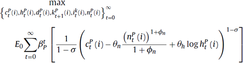
where Φn is the inverse of the Frisch labour supply elasticity, σ is the relative risk aversion coefficient and Θh and Θn capture the relative importance of housing and labour respectively in delivering utility to the patient household. As usual, this optimization program is subject to a budget constraint as follows:
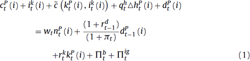
where  is the price of housing services,
  is the change in the stock of housing services, wt is the real wage,
  is the (predetermined) nominal interest rate on deposits, πt is the inflation rate,
  is the real rental rate of capital and
  and
and  represent the profits of the bank and the set of intermediate good producers, which both are assumed to belong to the patient households. The investment of household i in physical capital entails adjustment costs captured by the function
 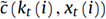 as follows:
with:

The conditions that characterize the solution to the optimization problem of patient household i are thus given by:
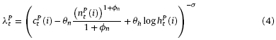


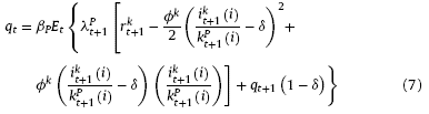
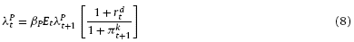
where qt is the Lagrange multiplier on the constraint given by the equation of physical capital accumulation (also known as Tobin's "q"),  represents the Lagrange multiplier of the budget constraint at time t. Eq. (4) corresponds to the standard Euler condition for consumption for a patient household. Eq. (5) determines the intertemporal, optimal demand for the stock of housing services. Eq. (6) corresponds to the traditional intratemporal labour supply schedule. Finally, Eqs. (7) and (8) establish the optimal condition for physical capital accumulation (net of adjustment cost) and savings. Notice that combining the latter two equations it is possible to derive a non-arbitrage condition in which deposits savings offer the same expected real return than physical capital.
3.2. Impatient households
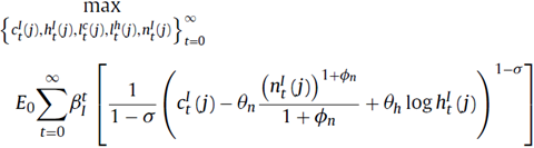
There is also a continuum of impatient households of mass 1 - µ. The relatively low discount factor of impatient households )  makes them willing to borrow for the sake of their consumption and housing plans. In this case, the objective of a patient household j is to choose sequences for consumption
  labour supply
  enjoyment of housing services (a stock,
  ), borrowing in consumer credit
  and borrowing in mortgage credit
  such that the following discounted sum of expected instantaneous utilities is maximized:
subject to the following budget constraint:
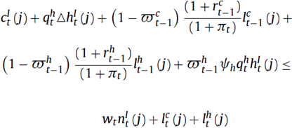
where  and
and  are the (predetermined) nominal interest rates on consumer credit and mortgage credit respectively,
  and
and  are the default rates of consumer credit and mortgage credit respectively, and Ψ
h corresponds to the recovery rate of housing services after default (that is, the share of the value of housing services that the bank can recover after default on mortgage credit). The left hand side of the budget constraint thus includes the repayment of loans from the previous period, taking into account that a fraction of loans will not be repaid and the payment that the bank recovers from the stock of housing services after default. This fraction, although endogenous as will be described below, is not a choice variable of the impatient household (that is, the impatient household takes
are the default rates of consumer credit and mortgage credit respectively, and Ψ
h corresponds to the recovery rate of housing services after default (that is, the share of the value of housing services that the bank can recover after default on mortgage credit). The left hand side of the budget constraint thus includes the repayment of loans from the previous period, taking into account that a fraction of loans will not be repaid and the payment that the bank recovers from the stock of housing services after default. This fraction, although endogenous as will be described below, is not a choice variable of the impatient household (that is, the impatient household takes  and
and  as given). Therefore, the model in this paper is not a model of the default choices/incentives of economic agents; it includes the default rate as a recognition of the fact that, in real life, the repayment of loans changes over time in a way that will depend on the aggregate state of the macroeconomy. Notice that consumer credit is unsecured so long as there is only a recovery value for mortgage default.
Borrowing from the impatient household is subject to borrowing constraints that establish limits for mortgage credit and for consumer credit as follows:


where mh and mc are maximum loan to value ratios for each type of mortgage credit and consumer credit respectively, both modelled as exogenous AR(1) processes. Mortgage credit borrowing is thus subject to a limit which depends on the expected, future value of the stock of housing services, whereas consumer credit borrowing is limited by the expected value of nominal wage income. The optimal conditions for the impatient household are given by:
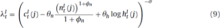
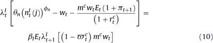
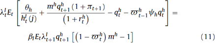
Financial frictions in the form of borrowing constraints affect in a substantial way the optimal allocation for the impatient household. Firstly, they distort the intertemporal consumption plan for impatient households, as can be seen from combining Eq. (9) with Eq. (10). Secondly, the borrowing constraint has an impact on the demand for the stock of housing services. In a frictionless environment, as shown by Eq. (5), the demand for housing services is determined by two interacting forces: A contemporary increase in housing prices reduces the demand for housing services; however, if the increase in prices persists over time, there is an incentive to demand more housing services since its value as a collateralizable asset rises. This effect is amplified by the fact that, when the borrowing constraint is binding, the pecuniary effect relaxes the limit, allowing the impatient household a smoother consumption plan. Finally, as is the case with models that include a labour supply choice and borrowing constraints, increases in the real wage relax the limit on consumer credit borrowing, which has an effect on labour supply which depends on the standard trade-off between income and substitution effects.
3.3. Firms
The model includes a continuum of producers of intermediate goods, each of them producing a different variety and operating under monopolistic competition subject to nominal rigidities. Intermediate good producers must borrow from the bank in order to finance working capital requirements. The set of intermediate goods is "bundled" together into a single, final good by a final good producer which operates under perfect competition.
3.3.1. The final good producer
There is a continuum of intermediate goods indexed by z ∈ [0, 1].The final good producer bundles together the output of these intermediate goods (denoted by yzt for every z at time t) into one single, final good whose output is denoted by yt. To this end, the final good producer employs a Dixit-Stiglitz aggregation technology:
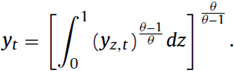
where Θ is the elasticity of substitution among intermediate goods. The final good producer takes as given both the price of each intermediate good pzt and the price of the final good pt when calculating the optimal demand for each intermediate good z. Thus, the optimization problem of the final good producer is given by:
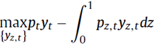
subject to the Dixit-Stiglitz aggregation technology. The first order condition of this optimization problem yields the standard demand curve for each intermediate good:

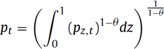
where Pt is the final good price index given by:
3.3.2. Intermediate good producers
Each intermediate good firm z utilizes labour (from both the patient and the impatient household) and physical capital to produce yz,t. In addition, intermediate good producers operate under monopolistic competition, and must therefore choose an optimal price for their individual varieties taking into account the demand schedule from the final good producer and subject to Calvo-style nominal rigidities. Thus, the problem of intermediate good producer z is two-layered: on the one hand, they must price their individual output; on the other hand, given their individual output, they must choose on the optimal use of capital and labour from each household. It is usually found easier to start with the latter problem.
Each intermediate good producer z combines patient and impatient labour and physical capital to produce their individual variety according to the following technology:

where kz,t and nz,t are the demands of physical capital and aggregate labour, respectively, and  is a technology process that follows an AR(1) process:

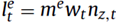
where a bar over a variable refers to its steady-state value. Labour from the impatient and the patient households are assumed to be perfect substitutes; in equilibrium, both types of households will earn the same real wage:  The intermediate good producer at this stage solves the standard, static, profit maximization problem taking into account a working capital constraint, which implies that the firm needs to borrow from the bank in order to finance the wage bill in advance (in what follows referred to as a business loan). The problem of the firm is as follows:

where me is the loan-to-value for business loans,  is the default rate on business loans, and
  is the (predetermined) real interest rate on business loans. In this case, the intermediate goods producer must finance a share 1 - me of the wage bill in advance using its own funds, and the remaining share using a business loan from the bank. Thus:
where  is the amount borrowed by the intermediate goods producer in the form of business loans. Similar to the case of mortgage credit, in the case of default the bank may recover some portion of the loan by going after the value of the physical capital stock the firm has rented from patient households. The corresponding recovery rate is given by Ψ
k. The optimal conditions for the intermediate goods producer are:
is the amount borrowed by the intermediate goods producer in the form of business loans. Similar to the case of mortgage credit, in the case of default the bank may recover some portion of the loan by going after the value of the physical capital stock the firm has rented from patient households. The corresponding recovery rate is given by Ψ
k. The optimal conditions for the intermediate goods producer are:
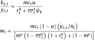
where mc t is the marginal cost of the firm expressed in units of labour.
The second layer of the optimization problem of an intermediate goods is the choice of an optimal price for their individual varieties. Price setting is subject to a Calvo-style nominal rigidity: each period, a constant fraction of intermediate good producers 1 - ε is allowed to choose freely an optimal price, whereas the remaining fraction 1 - ε must be content with the individual price of the previous period. The problem for each firm belonging to the first group is to choose an optimal price that maximizes the expected profit during the expected life of the chosen price, taking into account the demand function from the final good producer:
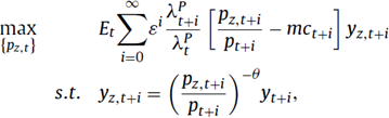
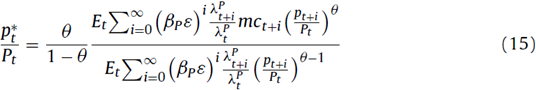
Where 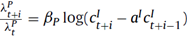 is the stochastic discount factor. The first order condition entails the standard, optimal pricing equation:
3.4. The Bank
The financial system is composed by a bank that intermediates savings from the patient households into credit to the impatient households and to the intermediate goods producer. The bank is assumed to operate under perfect competition (that is, the bank takes interest rates as given when solving its optimization problem). The objective of the bank is to maximize profits taking into account the demand for loans from households and firms and bank capital requirements set exogenously by the regulator. Profits are given by the difference between financial revenues plus recovered values after default and financial costs plus the penalty associated to the bank capital requirements. Financial revenues for each type of credit take into account the probability of repayment and are given by 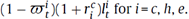
In addition to financial revenues, the revenue of the bank includes the liquidation (or recovered) value from the share of mortgages and business loans from that are not repaid. For the case of business loans, this recovered value is given by  with
with  , whereas for mortgages it is given by
The repayment rates (or default probabilities) are taken as given by all economic agents. These probabilities are endogenous and enter the model as a reduced form which depends on the output gap, a measure of the inverse of the leverage gap for each type of credit and an exogenous shock which is interpreted in the context of the model as a shock to the financial fragility of debtors:
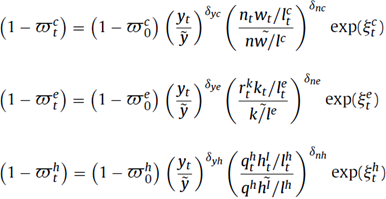
swhere a tilde over a variable denotes its steady state value,  represents the “financial fragility” shock for type of credit i and
  and
and  are fixed parameters. The shocks follow an AR(1) process with a common persistence parameter
  Notice that there is a different measure of the leverage gap for each type of credit: in the case of consumer loans, the reduced form includes the ratio between labour income and the size of consumer loans. In the case of mortgages, it includes the ration between the market value of the stock of housing services and the size of the mortgage loans. Finally, for business loans, it includes the ratio between the value of rented physical capital over the size of business loans.
The bank borrows from patient households in the form of deposits. Financial costs are thus made up of interest payments to depositors  . In addition to these financial costs, the model includes bank capital requirements as the sole macroprudential policy available to the policymaker. Specifically, this requirement is modelled as a penalty function that entails a cost to the bank that depends on the distance between observed bank capital and the minimum required. The minimum capital includes risk weights for each type of credit given out by the bank. The minimum, risk-weighted capital required from a bank is given by:

where σi, i ∈ {c, e, h} is the risk-weight attached by the regulator to each type of credit (which may be a function of repayment probabilities as well) and µv is minimum capital adequacy ratio. Given this minimum bank capital, the penalty function ΓKR that captures the requirement follows Den Haan and De Wind (2012) as follows:

where  is the observed bank capital and γ0, γ1 and γ2 are fixed parameters. The penalty function depends on the distance between
  and
and  , and the parameters of the penalty function are set in a way that the penalty function is asymmetric: as gets closer to
  the bank faces an increasingly prohibitive cost, whereas as gets further away from the bank receives only a tiny benefit. Taking all these elements together, the problem of the bank is as follows:
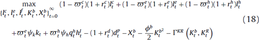
where  are retained earnings (investment of the bank in the form of bank capital) and
  corresponds to an adjustment cost to bank capital, which seeks to capture the idea that raising bank capital is costly. In a similar fashion than physical capital, bank capital accumulates according to:
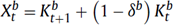
Finally, there is a balance sheet identity given by:

df + Kb = +/h + (19)
The first order conditions of the bank are therefor given by:
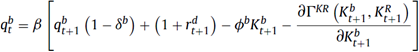
where  is the shadow price of the bank capital accumulation equation (a form of Tobin's "q" for bank capital) and there is an implicit arbitrage condition
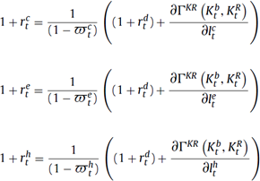
  . In equilibrium, interest rates for each type of credit must offset the expected opportunity cost of deposits (and Central Bank loans) and the marginal effect of each loan on the requirements of bank capital. In this sense, capital requirements affect the financial system along changes in the penalty function, which creates a pass-through effect on active interest rates.


4. Calibration
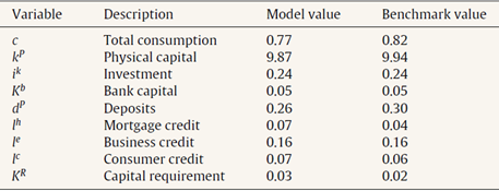
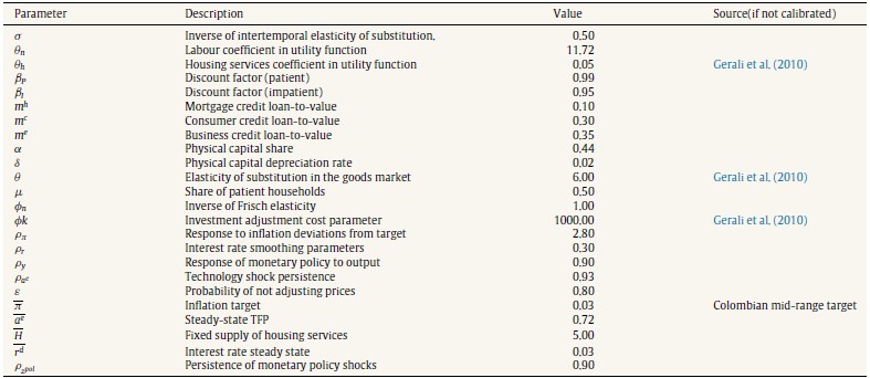
The parameters of the model are calibrated so that the steady state of the model replicates several quantitative properties of the real and financial sectors of the Colombian economy. Average, historical values of real and financial variables for the period between 1996 and 2015 are taken from DANE and the Colombian Financial Superintendency. Table 5 shows the values taken as a reference as steady-state values (as ratios of GDP) calculated by the model. Tables 16 and 17 at the end of the paper present the full set of values calibrated for the full set of parameters.
5. Results
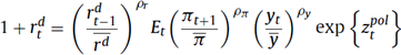
This section presents the set of responses of the equilibrium values of key variables of the model to three types of shocks: a monetary shock (one standard deviation to  ), a productivity shock (one standard deviation to
  ) and a financial fragility shock (one standard deviation to all
  ). The analysis of impulse-response functions contained in Tables 6-15 allows to study how the equilibrium relationship between the real economy and the financial system (the bank) changes in response to shocks. All impulse response functions spread over 50 periods of time and start at t=1, which is the time where the shocks are assumed to occur. The impulse response functions compare the calibrated version of the model with one where the capital requirement is eliminated (γ1= γ2 = 0). By comparing these two scenarios, it will be possible to discern whether the capital requirement help to deliver a smoother response of the economy to the shocks.
5.1 Productivity shock
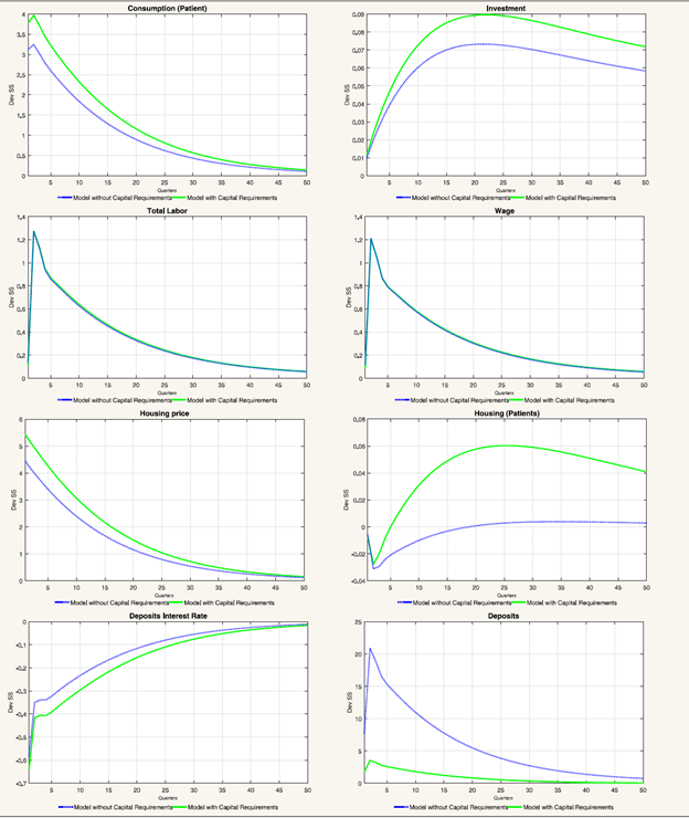
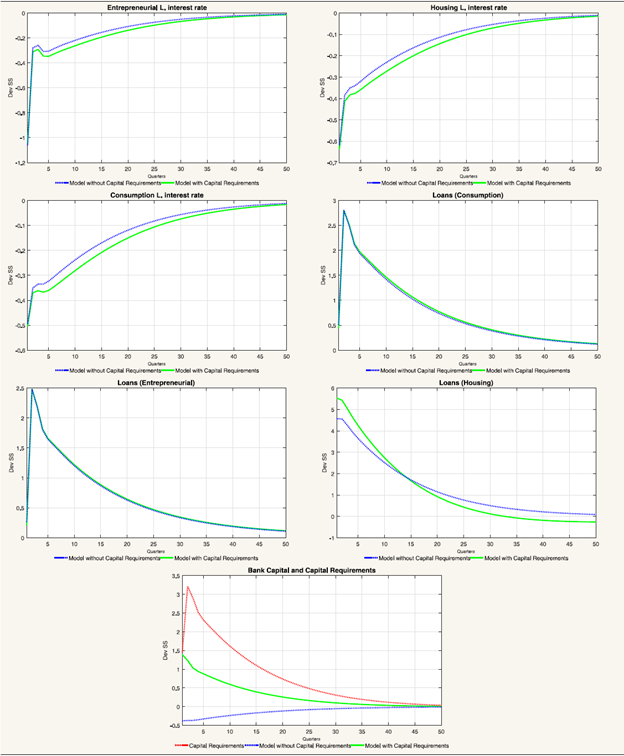
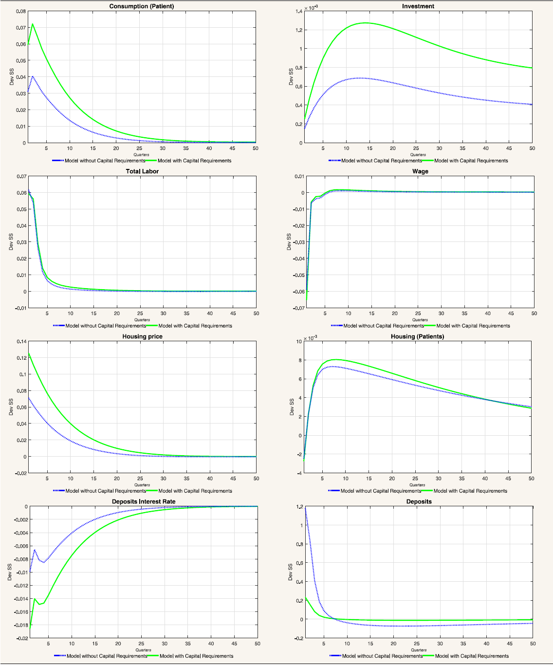
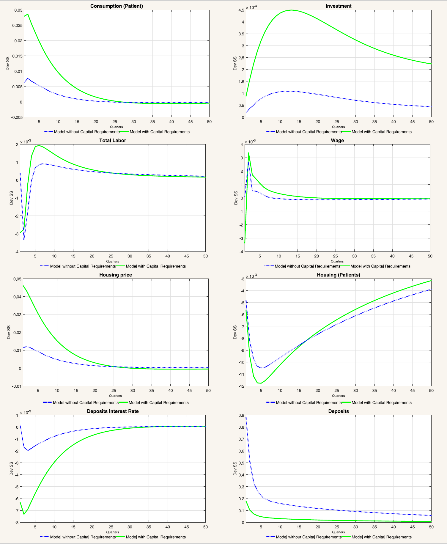
Tables 6 and 7 at the end of the paper present the impulse-response functions for a positive, one standard deviation shock to  . A positive productivity shock leads to the traditional hump-shaped response of investment and consumption (for both types of households) accompanied by a fall in inflation (unreported). Consumption increases following the increase in equilibrium labour, which is caused by an increase in the demand for labour from intermediate producers (the equilibrium wage increases as well). The price of housing services increases as the demand for them from the impatient household rises (as will be detailed below, mortgage loans increase sharply). Thus, there is a redistribution of the fixed supply of housing services from the patient households to the impatient households. Wealth effects of the productivity shock imply that deposits from the patient households increase at the same time as the equilibrium interest rate on deposits falls.
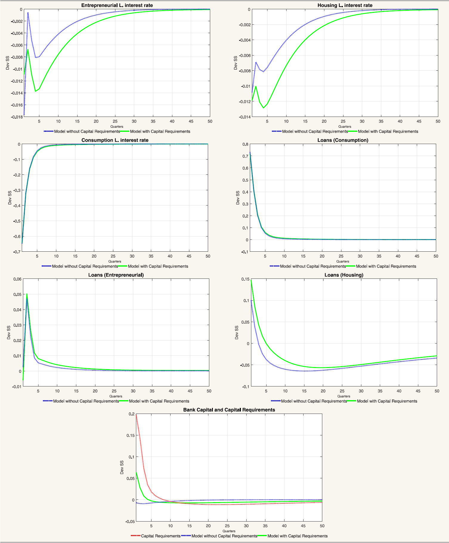
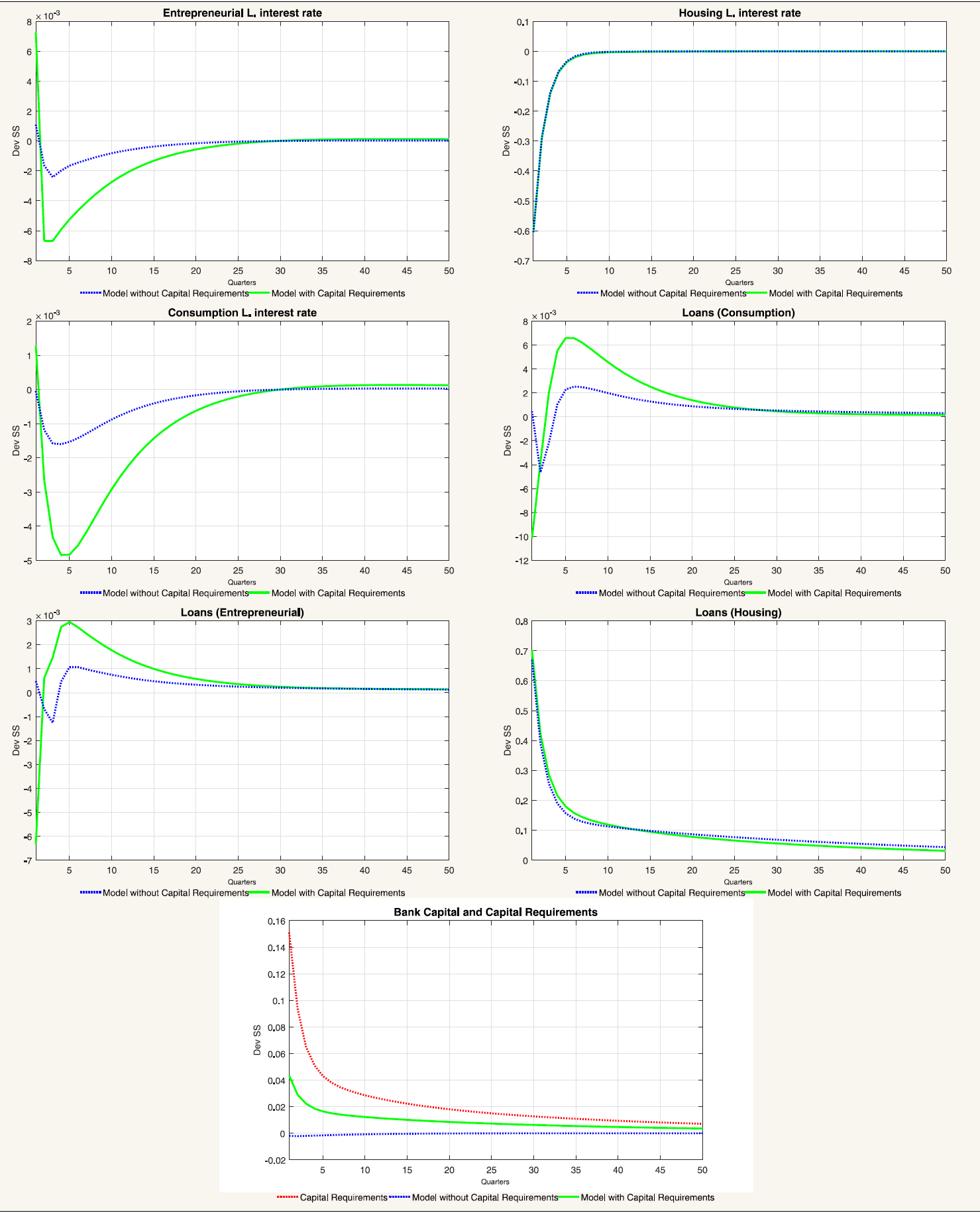
The fall in the deposit rate drives down interest rates for all credit categories (see the first order conditions for the problem of the bank). This is consistent with the observed increase in loans for all categories. Consumer credit follows closely the evolution of wages, which reflects the effect of an increase in the latter on relaxing the consumer credit borrowing constraint of impatient households. Similarly, business loans replicate the behaviour of labour and wages, reflecting the working capital constraint of intermediate goods producers. Finally, mortgages increase so long as the productivity shock relaxes the mortgage credit borrowing constraint of the impatient households (via a temporary increase in future housing prices).
The impulse-response functions tend to lend weight to the idea that capital requirements (as modelled in the paper) do not contribute to smooth the response of the economy to productivity shocks in terms of both real and financial variables. The response of bank capital and bank capital requirements offer insights into the effect of this policy tool on the response of the model economy. When capital requirements are absent, the bank substitutes its funding sources away from bank capital and into deposits: there is a huge increase in deposits when there are no capital requirements. The presence of capital requirements effectively limits the degree to which the bank can substitute funding sources: the increase in loans causes an increase in required bank capital (red line) to which the bank naturally responds by increasing bank capital. Thus, under capital requirements deposits do not increase by much (the demand for deposits is smaller) and therefore the fall in the interest rate on deposits is stronger than what would be observed where capital requirements absent. The stronger fall in the interest rate on deposits drives a stronger fall of interest rates for other credit categories, with the consequent impact on real variables and on the price of housing services.
5.2 Monetary shock
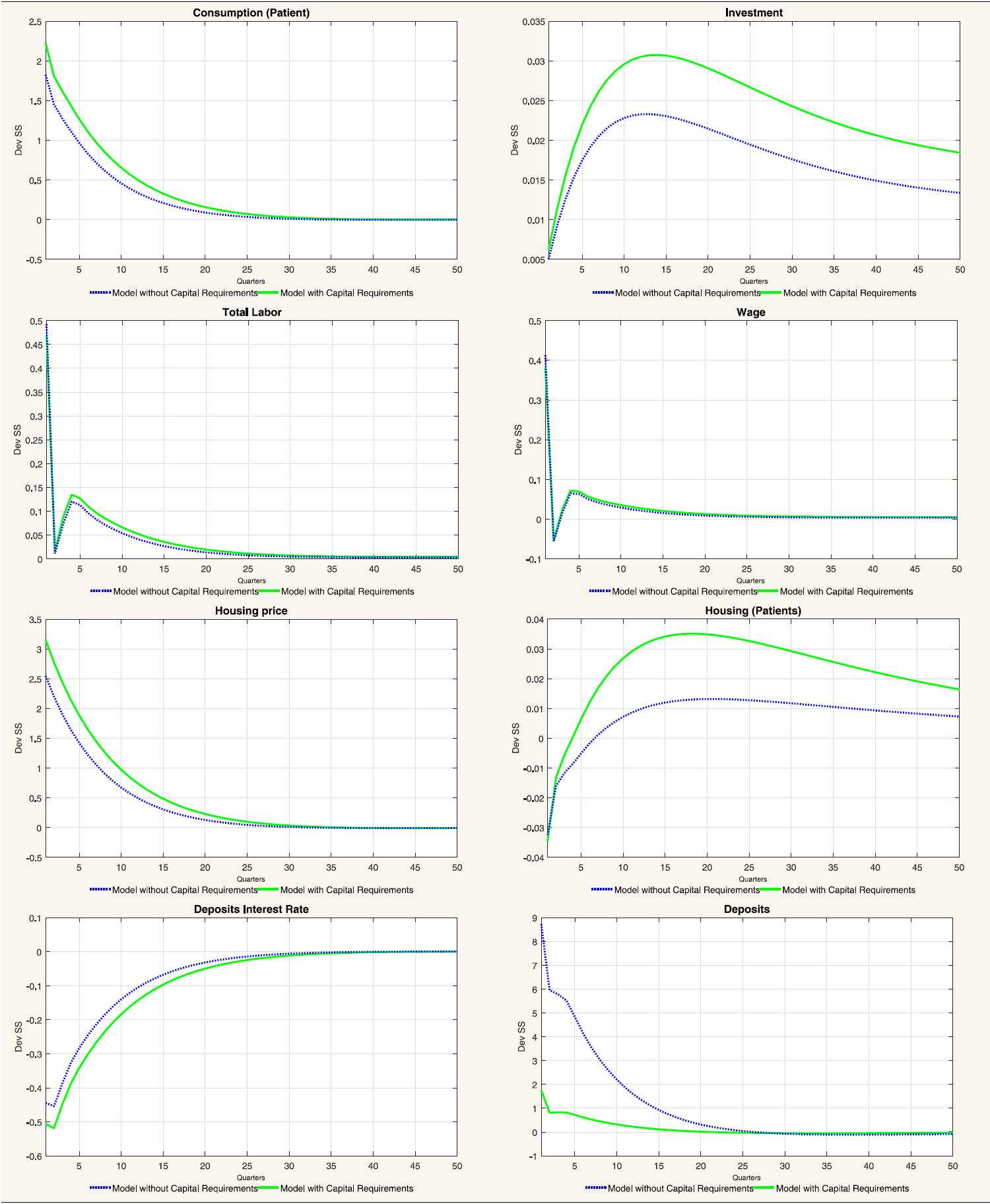
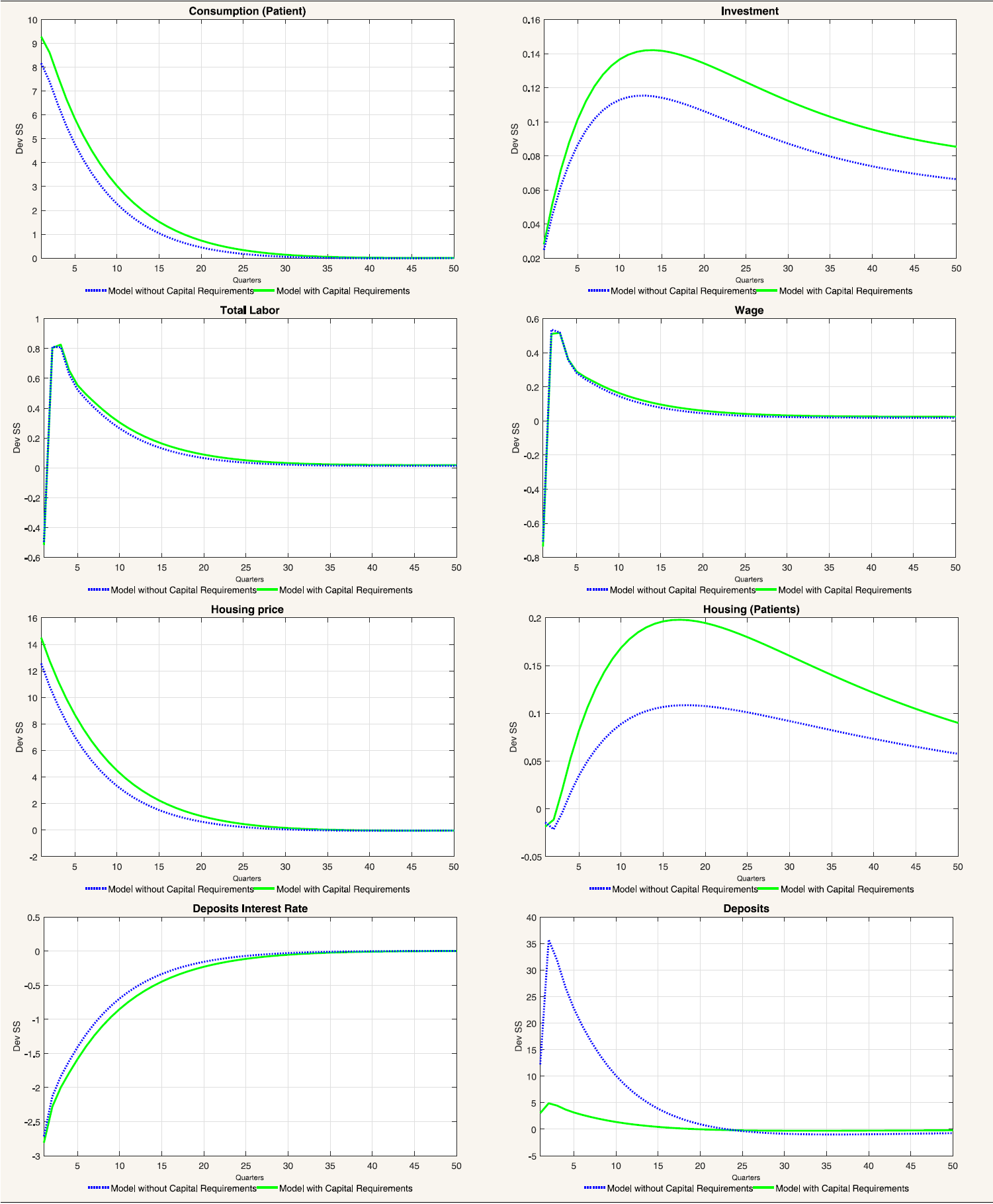
Tables 8 and 9 at the end of the paper present the set of impulse response functions to a negative, one standard deviation shock to  (that is, a positive or expansionary monetary shock). The response of aggregate variables such as consumption and investment is consistent with what is traditionally found for a policy shock. Inflation (unreported in the tables) increases on impact as expected, which induces an endogenous response in the policy rate. As is the case with productivity shocks, consumption tracks closely the behaviour of equilibrium labour and wages. Compared with productivity shocks, an expansionary monetary shock causes only a fleeting increase in the demand for labour, which is associated to a momentary increase in the wage rate. The increase in the demand for labour is caused by a relaxation of the working capital constraint for intermediate goods producers brought about by the reduction in interest rates, as will be discussed next. There is a similar redistribution of the use of housing services (and a similar response of the price of housing services) as was the case with productivity shocks, and for the same reasons.
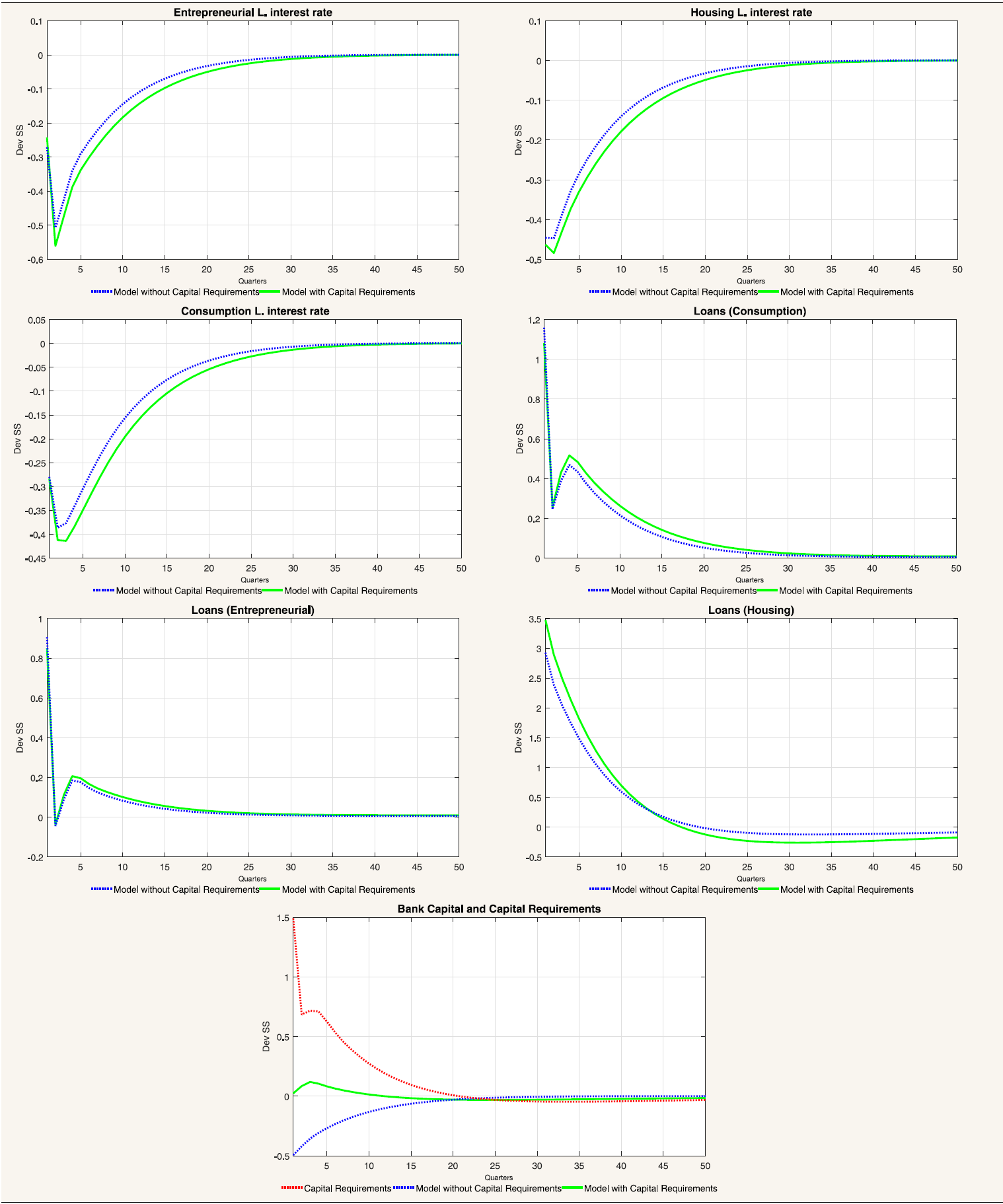
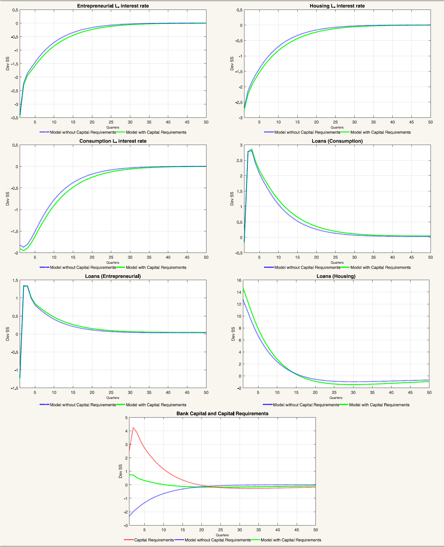
The response of interest rates is also akin to the one observed under productivity shocks, with the difference that the lower persistence of monetary shocks translate itself into brief responses of interest rates. Again, this is consistent with the observed, temporary increase in loans for all categories. Consumer and business credit follows closely again the evolution of wages and equilibrium labour, whereas mortgages increase following the increase in the price of housing services and the relaxation of the borrowing constraint.
The logic described above regarding the effect of capital requirements on the response of the model economy applies to monetary shocks in a similar fashion. Given that neither the cost of adjustment of bank capital nor the penalty function parameters change after a monetary shock, capital requirements have the effect of crippling the ability of the bank to switch to cheaper funding sources (deposits), which depresses the structure of interest rates, amplifying the response of all loan categories and thus, of consumption, investment and labour demand.
5.3. Financial fragility shocks
Finally, Tables 10-15 at the end of the paper present the set of impulse response functions to positive, one standard deviation shocks to  and
and  in isolation (in that order). The shocks are interpreted as exogenous increases in the probability of repayment for each of the three credit categories, or as positive financial fragility shocks.
With the exception of investment, the responses of both aggregate and financial variables exhibit wide differences across shocks to the fragility of different credit categories. The reason for these differences is apparent from the set of first order conditions of the problem of the bank: in a first round, increases in the probability of repayment of either credit category cause a fall in the interest rate of that specific credit category, and not of other categories. This is unlike the case with monetary shocks, which in principle affect the structure of interest rates of the economy in a similar fashion, as follows from the same set of first order conditions. This is evident in Tables 11, 13 and 15: the interest rate that reacts the strongest to the shock is the specific interest rate of the credit category subject to the financial fragility shock in either table. This effect causes expected differences in the responses of some aggregate variables: on impact, consumption increases the most on impact when there is a shock to consumer credit fragility whereas total labour increases the most when there is a shock to business credit fragility.

Shocks to financial fragility also differ inasmuch as they create negative wealth effects either on impatient households (in the case of consumer and mortgage credit) or intermediate good producers (in the case of business credit). These wealth effects arise from the fact that an increase in the repayment probability effectively increases the debt burden of households and intermediate good producers (see the optimization problem of either of these agents). In the case of a consumer credit fragility shock, this wealth effect incentivizes the household to increase labour supply (Table 10), which reduces the wage rate (unlike any other shock considered in this paper. When a shock to business credit fragility is considered, the wealth effect creates a reduction in the demand for labour (and the wage rate) on impact. Afterwards, consumption and labour exhibit a hump-shaped response (similarly to the case of productivity shocks), which arises from the fact that an increase in business credit fosters the ability of firms to finance labour and, therefore, to rent physical capital. Lastly, a mortgage credit fragility shock features interesting distributional implications. Firstly, the wealth effect of the shock forces impatient households to reduce consumption at the expense of patient households. The effect of the shock on total consumption is therefore mild. The opposite pattern is observed for the use of housing services: as the interest rate on mortgages falls, patient households enjoy lower housing services at the expense of impatient households.
Despite the diversity of responses observed under different categories of financial fragility shocks, capital requirements are again shown to amplify the response of the economy in a similar fashion. The mechanics of this result is common to all fragility shocks and to the aforementioned productivity and monetary shocks: capital requirements disrupt the ability of the bank to switch to deposits after a shock that reduces the deposit rate. The consequent reduction in the demand for deposits amplifies the effect of the shock on the deposit rate and on other interest rates, which magnifies the response of loans across all credit categories.
6. Concluding remarks
This paper presents a DSGE model with a bank and capital requirements calibrated for the Colombian economy. The model explores the interaction of real and financial variables taking into account multiple types of loans and the effect of required capital on equilibrium allocation. To understand the dynamic effects of capital requirements, we assess the impact of monetary, productivity and financial fragility shocks on the model economy. In general, capital requirements are found to be procyclical in the sense that they magnify the response of the economy to shocks of either type.
It is important to highlight that the transmission channel of macroprudential policy (capital requirements) operates through the interest rate for each credit category. This model is sufficiently flexible to consider alternative tools of macroprudential policy: one possible extension of the model would be to consider dynamic provisioning scheme or marginal reserve requirements to study its impact on the economy and its differences with conventional capital requirements. The comparison of the several macroprudential policies would help achieve a better understanding of the equilibrium interaction of monetary and macroprudential policies.

