English (pdf)
 Article in xml format
 Article references
 Send this article by e-mail
 Cited by SciELO
  Cited by Google
  Similars in
SciELO
Similars in
SciELO  Similars in Google
 Permalink
1 Introduction
The recent wave of austerity-focused fiscal policies in the Euro Area (henceforth EA) have casted doubts on the effectiveness of fiscal policy to counter busts and reduce economic uncertainty. The heavy focus on dynamically sustainable government budgets has both reduced the space and scope for governments to use fiscal policy in a discretionary manner, leaving room for rule-based fiscal policy-decisions. Moreover, in an environment of unconventional monetary policy, it is even harder to argue for the merits of conducting expansionary fiscal policy.
In the EA, there is the additional institutional complexity. While there is a unique monetary policy, the fiscal policy competence is still national and very diverse across the area member states. Besides, the institutional arrangements around the decision-making on fiscal policy are heterogeneous. While in fiscally conservative countries such as Germany, the decisions on government spending, revenues, and debt are almost apolitical and rule-based, in southern European countries such as Greece or Italy, they are entirely influenced by the political cycle, political interests and are highly susceptible to short-termism. As a result, the specific content of the spending-and revenue plans, the horizon of such policies, and the role of debt sustainability in constraining such decisions are very diverse across the member states.
Despite these large discrepancies, there is a rising interest in exploring whether there exists a common core in the fiscal policy-making in EA. In particular, is there a fiscal unity, either as a result of spill-overs from the monetary union, or as a result of (voluntary) convergence towards a fiscal paradigm? In other words, have criteria under the Maastricht Treaty aiming at fiscal prudency, the choice for German fiscal conservatism over the Southern European preference for fiscal discretion, or even the late austerity measures lead to the emergence of a common fiscal response despite the lack of a formal fiscal union? In the context of a possible future fiscal union, these questions are highly relevant, both from an academic and policy-focused optic.
But, beyond these European affairs, there are two other pressing concerns regarding fiscal policies and their impacts. The first (previously explored by Fragetta and Kirsanova (2010), Rossi and Zubairy (2011), and Gerba and Hauzenberger (2014), albeit mostly for the US) is the importance of including monetary policy actions for fiscal policy estimates, and the role of (implicit) monetary-fiscal interactions for economic stability. In particular, how stabilising is fiscal policy in a world of rule-based (conventional) monetary policy compared to a world of highly-expansionary bounded (unconventional) monetary policy? Is fiscal policy equally effective, or is fiscal expansion more effective when monetary policy is bound by the zero-lower-bound? Along the same lines, there is an increasing curiosity in understanding the impact of economic (and financial) uncertainty on their joint policy effectiveness. Here, the European case is especially relevant since EA has experienced both uncertainties since the onset of the Great Recession. Initially the uncertainty came from the financial sector. However, as concerns regarding the sustainability of budgets for several southern European economies rose, the uncertainty switched mainly to (macro)economic. What's more, the bail-out of many banks in the EA meant that the nexus between the fiscal-economic-financial aspects became even tighter.
The current paper attempts to answer some of these concerns. In particular, I attempt to provide answers on the existence of a common fiscal policy in the EA since 1980's. whether and how these have interacted with monetary policy, the degree of effectiveness of fiscal policies in normal vs. turbulent (or uncertain) times. To answer these questions, I cast our fiscal, monetary and macroeconomic variables in a Structural Bayesian Vector Autoregressive (S-BVAR) framework and model the structure using theory-based sign-restrictions discussed in Gerba and Hauzenberger (2014). I estimate the model using the penalty function-based approach instead of the pure exclusion-based one used in many models with sign-restrictions. I opt for this approach because it is much more information-intensive, data-driven, and holistic.
On the questions regarding a common fiscal reaction (or response) in the EA, I find affirmative evidence. I identify EA-wide shocks and find statistically significant (endogenous) responses of fiscal policies to shocks. While spending policy responses are truly discretionary and independent, I find that tax responses are highly cycle-driven and dependent. I also find significant evidence for interactions between fiscal-and monetary policy. Said that, the nature of interactions depends very much on the shocks that hit the economy. While for a spending and monetary policy shock they act as substitutes, they act as compliments for a business cycle shock. At the same time, the way the two fiscal policies interact with monetary policy is also different and independent of each other. On the effectiveness of fiscal policies, we find that the spending multiplier is higher than the tax multiplier. Nonetheless, their relative efficacy has changed over time, with the spending (tax) multiplier falling (rising) since the onset of the Great Recession. I also show that it is crucial to include government debt in the estimation of monetary-fiscal interactions. Failing to recognize the debt channel of fiscal-and monetary policies will result in misinterpretations of the estimates. To conclude, there are considerable differences in the nature of monetary-fiscal interactions between the EA and the US. Not only are the impulse responses to different shocks significantly different between the two economies, but also the fiscal multipliers vary a lot. Standard Keynesian (or spending-oriented) fiscal policy is more effective in expanding output in the Euro Area while tax reductions are more effective in the US.
The paper makes four important contributions. First, it studies the question of monetary-fiscal interactions from an empirical perspective. Most of the literature, even in the US, has generally been based on DSGE models (or similar). The number of empirical studies on this topic are fewer (some of the exceptions are the studies cited above), and even more so for the EA. Second, as far as I am aware, there is no other paper that examines fiscal policy, fiscal multipliers and policy interactions in EA stretching as far back as in this paper. The sample period covered here covers important episodes such as the Great Stagflation, Great Moderation, Great Recession, the introduction of the Single Market and later the Euro, and unconventional monetary and fiscal policy. Third, I separately examine spending and tax multipliers, and systematically compare those to individual member state estimates found in the literature. Most of the studies on EA either treat the two multipliers as one or estimate only one of the multipliers (Alloza et al, 2017), use a much shorter sample period, or produce biased estimates by ignoring the interaction with monetary policy. On top, there are many more studies that examine the multipliers of the individual member states than for the entire EA. Fourth and last, I apply a robust identification scheme to jointly identify fiscal-and-monetary policy shocks in an econometric framework. Besides Rossi and Zubairy (2011), Franta et al (2012), and Gerba and Hauzenberger (2014), I am not aware of other studies using the full empirical identification strategy to examine interactions. Different to these papers, however, I apply this framework on EA, meanwhile they do so for the US, or other countries.
2 Econometric approach
In the following sections, I will briefly describe the econometric method used to estimate the policies jointly in a macroeconomic structural BVAR, based on sign restrictions. Full technical details can be found in the Appendix.
2.1 VAR models
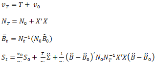
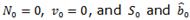
I follow Uhlig (2005) and Mountford and Uhlig (2009) in defining our BVAR model. Further details can be found in the appendix. I start with a generic reduced-form VAR model:

where  is an mx1 vector of data at date
  is a constant of size
  are mxm coefficient matrices and u
t is a one-step ahead prediction error with
are mxm coefficient matrices and u
t is a one-step ahead prediction error with  its variance-covariance matrix.
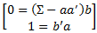
Let  be the normalized eigenvectors of Σ and
  be the corresponding eigenvalues. In addition let a be a vector. Then there are coefficients
  such that:

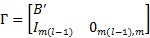
Vector a is thus an impulse vector, i.e. it can be shown that there exists A such that AA ̀=Σ and so that a is a column of A. In this vector, there are m-1 degrees of freedom in picking an impulse vector, and so they cannot be arbitrarily long.1
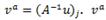
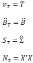
Next, we wish to compute an impulse response given the impulse vector a. Let 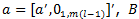 is the VAR coefficient matrix, and
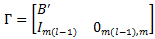
and compute 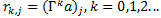 to get the response of variable j at horizon k. The variance of the k-step ahead forecast error of the impulse vector a is obtained by simply squaring its impulse responses. Moreover, summing over all aj, with aj being the j-th column of some matrix A (A;A = Σ) delivers the total variance of the k-step ahead forecast error. Finally, we assume that the errors u are independent and normally distributed.
The exact content of our impulse response vector to each and every shock will be defined below. The four fundamental shocks we consider are: spending, taxes, monetary policy, and output (or business cycle).
2.2 Identification scheme
I use sign restrictions, summarized in Table 1, and outlined in Gerba and Hauzenberger (2014) to identify jointly four orthogonal shocks: a business cycle shock which increases output and taxes; a monetary policy shock which increases the interest rate and decreases inflation and output; a spending shock which increases spending, debt and output; and a tax shock which increases taxes and decreases debt and output. All restrictions must hold for one quarter, except for the responses of the variables which are directly associated to the shock (e.g. tax shock on taxes), which must hold for four quarters. Having somewhat longer restrictions here rules out transitory effects.
The theoretical considerations behind our choices are relatively uncontroversial and consistent with most dynamic general equilibrium (DSGE) models that include monetary-fiscal interactions as well as Keynesian aggregate supply and demand diagrams.2 However, I did not want to be too restrictive in my choice of restrictions following just one DSGE model, since that would reduce the marginal contribution of data to my model. There is an intrinsic trade-off in choosing the sign restrictions, similar in general to Bayesian estimation. On one hand, tight sign restrictions improve identification and reduces the model space (or removes undesired models). On the other, it constraints the data input in the estimation procedure and strains the algorithm. Hence, there is an important balance to strike. I therefore choose restrictions that are in line with many (if not most) structural models including monetary-fiscal interactions, but allow sufficient flexibility to allow the data to determine the best-fitting model.
Table 1 Imposed Signs on the Impulse Responses
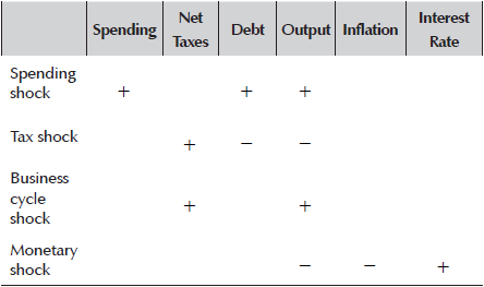
Note: A blank entry indicates no restriction on the specific combination of shock and response. For the estimations without debt in the model, debt sign-restrictions do not apply.
Source: author’s calculations.
In addition, my restrictions discard more controversial phenomena such as expansionary fiscal contractions see, e.g. Giavazzi, Jappeli and Pagano (2000) or the price puzzle. At the same time, with my choice of restrictions I avoid some issues often criticized in the structural VAR literature. For example the missing link between theory and a simple Cholesky decomposition, or the weak information provided by sign restrictions if one takes a too agnostic view on the identification of shocks see, e.g. Canova and Paustian (2011). Being too agnostic may have especially severe consequences if the relative variance of the shock of interest delivers a weak signal. The usual suspect here is the monetary policy shock. So the relatively large number of theory driven restrictions should a-priori lead to a good performance and reliability of my approach.
Although it is not of my primary interest, identifying a business cycle shock is crucial to adequately track the source behind the fiscal shocks, especially on the tax side. Otherwise I cannot disentangle whether a change in taxes comes from fluctuations in output or a tax shock see, e.g. Blanchard and Perotti (2002) or Mountford and Uhlig (2009). Just as a remark, I do not differentiate between a demand driven or supply driven business cycle shock; the results will, however, provide an indication of the relevant driver in a particular regime.
2.3 Estimation procedure
Numerically, the penalty function approach is implemented in the following way. For more details, see the appendix, Uhlig (2005) or Mountford and Uhlig (2009).
First I define a penalty function:
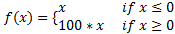
The function penalizes positive responses (negative for spending shock) in linear proportion and rewards negative (positive) responses, albeit with a weight 100 times smaller than the positive (negative) penalties.
Next, I draw the parameters (B, Σ) from a Normal- Wishart prior.
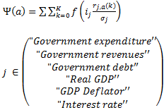
Let 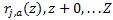 be the impulse response of variable j, and σ
j
its standard deviation of the first difference of the series for the same variable j. In addition, let ι
j
= -1 if j is the index of a variable x in the data vector, for instance the interest rate, and ι
j
= 1 otherwise. Then, the monetary policy impulse vector a4 is the one which minimizes the total penalty function Ψ(a), which penalizes positive impulse responses for output and inflation at horizons k = 0 and k = 0, 1, 2, 3 ,4.
be the impulse response of variable j, and σ
j
its standard deviation of the first difference of the series for the same variable j. In addition, let ι
j
= -1 if j is the index of a variable x in the data vector, for instance the interest rate, and ι
j
= 1 otherwise. Then, the monetary policy impulse vector a4 is the one which minimizes the total penalty function Ψ(a), which penalizes positive impulse responses for output and inflation at horizons k = 0 and k = 0, 1, 2, 3 ,4.
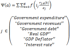
Along the same lines, the tax impulse vector a2 is the one that minimizes the total penalty for positive impulse responses of debt and output. On the contrary, spending-and business cycle impulse response vectors a1 and a3 are the ones which minimize a penalty function penalizing negative impulse responses of debt and output for spending shock, and output only for business cycle shock.
This penalty function is asymmetric insofar it punishes violations a lot more strongly than rewarding large and correct responses. Second, it is continuous in order to make the standard minimization procedure viable. Third, the penalty function punishes all deviations, but not equally. In its current form, even small violations of the signs are punished. However, larger deviations are punished more than smaller ones, and so there is also magnitude discrimination.
To draw inference from the posterior, I employ the Monte-Carlo method and take n draws from it. I set n = 20,000 and keep n = 10,000 out of these in order to strike a balance between higher numerical accuracy and time consumption from optimizing over the shape of the impulse responses. For each of these draws kept, I calculate the impulse responses and the (forecast error) variance decomposition, and collect them. Hence in total there are 10.000 draws for each point on an impulse response function, which allows me to easily calculate the 95% error bands.
2.4 Data
The data sample consists of 6 variables: government expenditure, net taxes, government debt, real GDP, GDP deflator, and the short-term interest rate. Government spending includes both government consumption expenditures and gross investment, and net taxes are the current receipts less net transfers and net interest paid. On the nominal side I measure prices with GDP deflator and use the 3-month EONIA rate as the short-term interest rate. The three variables on the real side of the economy enter the VAR as logarithms.3 For the pre-2002 period, the data have been backward extrapolated by the ECB and an EONIA-equivalent rate had been used for the short-term interest rate. In addition for the fiscal variables, the data have been aggregated using the method of Eurostat. Further data description, including the extrapolating method used can be found in Paredes et al (2014).
Table 2 reports descriptive statistics of the data. Most of the data distributions are symmetric, with a high probability mass around the mean, and low tails. The only exception is the interest rate, with a standard deviation almost as high as the median. Hence the distribution is quiet disperse, possibly capturing the high variation in interest rate levels during the extreme periods of turbulence from monetary targeting in early 1980's, and the zero-lower bound since the Great Recession.
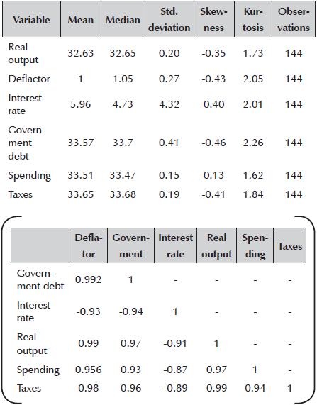
Likewise, the contemporaneous correlations of the different variables are in line with the priors in the literature. Variables which have been identified in the literature as having strong positive correlation, such as output and government debt, output and GDP deflator, or government spending and debt, also have high (positive) correlations in my simple matrix below. Note the surprisingly high correlation between interest rate and government debt, at -0.93. It means that there are strong interactions between government financing and the monetary stance in the EA. When interest rate is low, a lot of new government debt is accumulated, and vice versa.
But so far, the discussion has only concentrated on the superficial relation between the variables. To get a better idea on the causal relation between them, I perform a sequence of one-and two-sided Granger causality tests. Results are reported in Table 3. A star (*) means that the statistic is significant at 10% level, and thus variable x Granger causes variable y. The relationships in bold are the ones of particular interest since they represent the direct interaction between monetary and fiscal policies. The number of lags included in the estimation of the pairwise Granger causality test is 4 since the frequency of the data is quarterly. In the one-sided causality tests, I find sufficient evidence for Granger causality between the fiscal and monetary variables. In particular, the two fiscal variables (spending and taxes) Granger cause each other, as do interest rate and taxes. At the same time, I find that government debt Granger causes taxes, but that spending Granger causes debt. Hence, while spending decisions determine debt, debt acts as a constraint on the tax decisions. In the two-sided test, I however find that the bidirectional causal relation exists between interest rate and spending. In sum, even in the raw data (without imposing any structural relations), I find sufficient evidence of monetary-fiscal interactions. This serves as sufficient motivation for exploring further this joint relation in a structural model.
Table 3 Granger causality tests
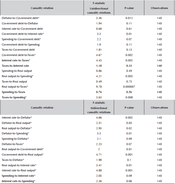
Note: A star (*) means that the statistic is significant at 10% level, and thus variable x Granger causes variable y. The relationships in bold are the ones we are in particular interested in as they represent the direct interaction between monetary and fiscal policies. The number of lags included in the estimation of the pairwise Granger causality test is 4 since the frequency of the data is quarterly (so to capture the lagged annual relation).
Source: author’s calculations.
3 Results
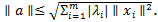
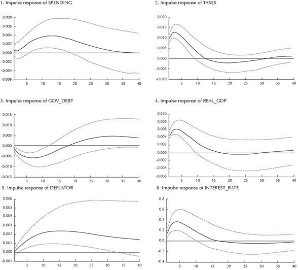
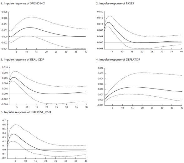
The lag length test found the optimal length to be 2. I run 20.000 Markov Chain Monte Carlo simulations and save 10.000 for inference. These parameters are relatively standard in the literature and allow for sufficient draws in order for the routine to converge.4 I let the number of subdraws for sign restrictions to be 2.000 so that 10 draws in each subdraw are included. Once the algorithm has converged and the routine has completed, we calculate the impulse responses with 95% confidence intervals (in red), and the (forecast error) variance decompositions. The IRFs are reported in Appendix A 5
The discussion of the results is organized in the following way. Section 3.1 discusses the responses to fiscal and monetary shocks in the benchmark model. I continue by analyzing the fiscal multipliers for EA in Section 3.2 and compare those to those found for the individual member states in 3.3 (and 3.9). In Section 3.4 I take a closer look the contribution of the shocks in explaining the fluctuations in each of my variables through forecast error variance decompositions. I combine all this information in determining the degree of monetary-fiscal interactions in 3.5. The last five subsections are then dedicated to various extensions. First, I compare my estimates to the ones obtained in a model without debt in 3.6. Next, I evaluate the evolution of coefficients over time in 3.7. I compare my interaction results for the EA to the ones obtained for the US in 3.8. 3.9 is dedicated to the comparison of tax multipliers within EA, and 3.10 is dedicated to a series of important robustness checks (pure sign restrictions, alternative identification schemes, estimation in growth rates, and comparison of results to a model identified using a recursive scheme.
Before the discussion, I would like to introduce the concept of policy interaction I will be making use of throughout the subsequent sections. If fiscal and monetary policy exhibit a positive or negative correlation implying that one policy responds (strategically) to the actions of the other, I say that the two policies interact or coordinate. Going one level deeper, and following Muscatelli et al (2004), if the interaction is such that both policies are expansionary I define them as being compliments. If the two policies move in different directions they act as substitutes. Finally, the last level of policy analysis regards the responses of the two policies to innovations in output, as in Melitz (2002) and Muscatelli et al (2004). If the interest rate rises after a business cycle shock, I say that monetary policy acts in a stabilizing fashion. Likewise, if taxes rise or government spending falls, I equally say that fiscal policy enhances output stability. Since I superimpose, via my identification scheme, that taxes will always rise following a positive business cycle shock, the final outcome on the fiscal side will therefore depend on the sign and the magnitude of response of government spending.
Judging from Appendix A on the impulse responses to all the four identified shocks, I find sufficient evidence for interaction between the two policies. In all cases, except for a tax shock, both the monetary policy and the two fiscal policies react, either in the same or in the opposite direction. Moreover, in all cases except for a tax shock, the correlation of the two fiscal policy responses is positive.
3.1 Benchmark monetary-fiscal shocks
Digging a level deeper on the interaction (or coordination) between the policies, the findings are even more interesting. Commencing with the reaction of monetary policy to a spending shock in Table 4 shows that the two policies act as substitutes. Interest rates increase by about 0.2 percentage points to accommodate the demand-side expansionary effects of the increase in spending. Note, however, that because of this strong monetary policy response, actual inflation does not increase very much as the response of interest rate is already accounted for in the actual inflation. Expected inflation, on the other hand, increases by more, as is indicated by the output response. This is probably the reason for why interest rate responds so strongly, since the expansionary effects from a rising output raise expected inflation, which triggers a strong reaction of the central bank.6 As a result, fiscal expansion has been accompanied by a monetary contraction. This pattern is in line, for instance, with the New-Keynesian DSGE model of Corsetti et al (2011), but differ from Mountford and Uhlig (2009). However, their estimates are based on data for US and over the period (1955:I to 2000:IV), thus quite different to these.
Table 4
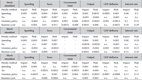
Note: The left (vertical) column reports the shocks identified, and the right (horizontal) row are the variables responding to one standard deviation shock. The magnitudes are interpreted from the impulse response functions reported in Appendix A and B. N.S. means that the responses are not statistically significant at 95% level. Conversely, all reported values are significant at p=0.05.
Source: author’s calculations.
In response to a tax increase, on the other hand, the response of monetary policy is not statistically significant at 95% level. The reaction of inflation is weakly positive, while that of debt, spending, and (to limited extent) output is negative. Remember that these are fiscal policies beyond the automatic stabilizers (which will be captured by the reaction of fiscal policy to a business cycle or monetary policy shock). Note also how the confidence intervals are larger for spending, output and interest rate following a tax shock compared to a spending shock. Taken together, the results indicate that spending decisions are truly discretionary and independent, which in turn trigger a solid reaction from the central bank. Taxes and tax shocks, on the other hand, depend intrinsically on the state of the business cycle, and respond passively to output. The variance decomposition results in Table 6 seem to confirm this pattern. This is additional evidence for why the two fiscal policies should be considered distinctively.
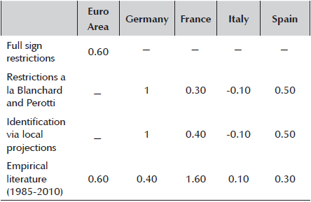
Table 6 Variance Decompositions: Specifications with debt
Note: Posterior means of the percent of forecast error variance attributed to the four shocks.
Source: author’s calculations.
To sum up the discussion so far, I find evidence of two things. First, interest rate seems to respond to output insofar that movements in output change inflation expectations. Second, my analysis provides additional evidence that the two fiscal instruments should be considered separately and distinctively. Apart from having strategic interactions between them, they also provoke distinct responses in monetary policy. Hence, it is possible that the central bank discriminates between the two policies, since spending increases have stronger expansionary effects on output.
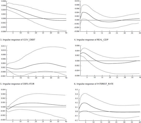
Next, let me turn to the transmission of monetary policy. Both fiscal policies react to the contraction caused by an interest rate rise, but in very distinct ways. While spending policy reacts as a compliment to a monetary contraction by also contracting, tax policy reacts as substitute by accommodating. Remember that no restrictions are placed on fiscal policy, so the responses are entirely data-driven. At the same time, debt seems to initially expand when net taxes drop, but then it recovers. Taken together it is highly probable that taxes initially respond because output contracts, following the monetary policy shock. Because taxes respond to business cycle movements (see variance decomposition of taxes), they fall significantly. However, the consequence is a surge in debt. Thus, in order to counteract this debt increase, spending also falls (after horizon 3). Output recovers, and inflation expectations turn positive. In this case, the fiscal authority seems to react in a passive way, first as a result of a contraction in output, and then to counteract the surge in debt. Muscatelli et al (2004) reach the same conclusion for the US regarding the initial fiscal expansion following a monetary contraction, but do not find the strong counter-reaction of fiscal policy further ahead in time in order to stabilize debt as we find for the EA.
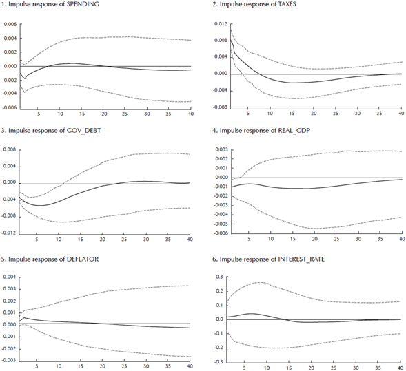
Finally, I go one level deeper and discuss the degree of policy interaction when the shock is not engineered by any of the two authorities (i.e. spending, tax, or monetary), but comes from outside in the form of an economy-wide business cycle shock. In Table 4, I again observe distinct responses of the two fiscal policies in relation to monetary policy. While tax policy complements the monetary policy contraction by increasing 0.0125%, spending substitutes (or counteracts) this contraction by increasing by 0.004%. Adding the two fiscal policy responses shows that the final fiscal stance is contractionary, since taxes rise more than spending, and so the fiscal policy acts as a compliment to monetary policy, just as in Muscatelli et al (2004) for the US. Moreover, both fiscal and monetary policy reacts in a stabilizing way to output. However, as in Melitz (2002), I find that government spending (contrary to taxes) reacts in a destabilizing fashion to innovations in output since, via the demand-side expansion, it attempts to push output further away from its steady state level. Net stabilization of the fiscal side therefore only occurs because of a larger reaction of taxes than expenditures.
3.2 Fiscal multipliers
To calculate the fiscal multipliers, I first need to convert the coefficients in Table 4 from responses of one standard deviation shock in spending and taxes to to multipliers. To do so, I transform the initial estimates of the variables in log-levels (output, spending and taxes) from elasticities into derivatives by multiplying them with the prevailing ratio of the responding and shocked variables. These transformed variables become "dollar deviations from trend" and can therefore directly be interpreted as multipliers (see e.g. Blanchard and Perotti (2002) or Kirchner, Cimadomo and Hauptmeier (2010)).
After conversion, I get that the spending multiplier for the full sample period is 0.60 and the tax multiplier for the same period is 0.50. First thing is that both multipliers are below 1 for the EA. This means that a smaller proportion of the public budget spending results in macroeconomic expansion. Second, the spending multiplier is higher compared to the tax multiplier. This implies that spending rises are more effective in expanding output compared to tax cuts.
Another interesting finding is that as soon as I do not control for debt in my model, the fiscal multiplier increases. In the specification without debt, the spending multiplier is 1, meanwhile that of taxes remains at 0.50. This means that if I do not include the costs from a less sustainable public finance in my considerations of the expansionary effects from a spending increase, I might upward-bias my estimate by overstating its impact on output.
Investigating further in-depth whether those multipliers had evolved over time, I find the following. First, the spending multiplier is consistently higher than the tax multiplier. Second, spending policies are more effective in expanding output during less turbulent times when less uncertainty prevails. To put the numbers into perspective, while in the pre-2008 sample, the spending multiplier was 0.8, it decreased to 0.5 in the sample up to 2010Q1, and then further to 0.42 in the sample up to 2011Q2. Taking into account that in the full sample, the spending multiplier was 0.6, this means that during uncertain times, such as during the financial-and sovereign debt crises, the effects of spending policies on output were significantly lower. On the other hand, during more 'normal times', such as in the pre-financial crisis world before 2008, or the post-sovereign debt crisis world after 2014, the expansionary effects from spending policies were much stronger. Hence, uncertainty plays a significant role in the efficacy of spending policies. Third, the tax multiplier has evolved in the opposite direction. It was higher during more turbulent compared to less turbulent times. While in the pre-2008 sample it was as low as 0.29, it increased to 0.375 in the sample stretching to 2010Q1, and even further to 0.41 in the sample up to 2011Q2. Forth and final, during the latest sovereign debt crisis, the spending and tax multipliers became roughly equivalent and very low, with the spending multiplier at 0.42 and tax multiplier at 0.41. This means that during the fiscal stress of 2011, it did not matter how the expansionary fiscal policy was executed, the macroeconomic effects were weak. Hence, our last finding is that during fiscal distress, the expansionary effect from fiscal policies is weak, no matter if the expansion was spending-or-tax driven.
Recent papers in the literature have emphasized the non-linear nature of fiscal multipliers during expansions (or normal times) and recessions. Using a regime-switching SVAR, Auerbach and Gorodnichenko (2012) find that the multipliers in recessions can be up to 4 times higher than during expansions. Baum and Koester (2011) and Baum et al (2012) find similar results for Germany and Japan. Similar discrepancies between the multipliers are also found in new-Keynesian DSGE model, such as Corsetti et al (2010) and Erceg and Linde (2012). While I do not perform a full TVP-VAR estimation in this paper, I can effectively discriminate between calmer and more turbulent times since the Great Recession. My results confirm partially the results in the literature. While tax multiplier became much higher during the crises periods, the spending multiplier is higher during less turbulent (or normal) times. There might be several reasons for some of this discrepancy in results. We treat the two fiscal instruments as independent measures while several others only look at the total fiscal stance. Our time-varying exercise focuses on the period of zero-lower-bound (ZLB) of monetary policy while the previous studies capture mostly the pre-ZLB period. Lastly, because EA has a distinct fiscal set-up to most other countries, there may be significant differences in the multipliers owing to institutional differences with other countries such as the US, Japan, or even Germany.
To conclude this section, I find that spending increases is more effective in expanding the (short-term) EA output than tax decreases. However, the effects are highly non-linear. During period of high uncertainty, the tax-oriented expansionary policies become marginally more effective, while during tranquil periods, fiscal policies focused on spending are significantly more effective (up to 3 times). Lastly, during times of fiscal distress, both policies are equally ineffective in expanding output, with spending increases half as effective compared to the pre-2008 sample.
3.3 Spending multipliers across the Area
One valid criticism of the identification strategy applied so far is that I assume that the economic structure between the countries in the EA are the same, which produces an identical fiscal policy innovation across, and which interacts with a common monetary policy of the ECB. Nonetheless, the recent sovereign debt crisis in Europe showed that the countries of the union remain very diverse in their economic structure, and thus also the transmission of policies. Therefore aggregation of behavioural equations across countries that have different parameters may produce a bias in the aggregate model.
To overcome this problem, I will compare my estimates for the aggregate EA for those found for the 4 largest economies inside it: Germany, France, Italy, and Spain (Alloza et al, 2017). The sample on which these estimates were based on is identical to the one used in this paper, stretching from 1980-2015. Moreover, the identification of fiscal shocks is based on the identification strategy of Blanchard and Perotti (2002), which is similar to ours. In addition, for robustness purposes they re-run the same model but using local projection method as their identification strategy. The only difference with ours is that they do not include monetary shocks in their model. However, since the focus in this section is on the distribution or heterogeneity of fiscal shocks across the EA, we can omit the common monetary policy for the moment.
The first thing to note from Table 5 is that the spending multiplier indeed varies significantly across countries. While in Germany spending policies are very effective and generate an equiproportional increase in GDP, on the other end in Italy, it results in a decrease in GDP. Nonetheless, all multipliers are strictly below or equal to 1, which is in line with my qualitative findings for the Area as a whole, and in line with more conservative multipliers found in the literature. Spain seems to be the closest to the average EA estimate.
Second, there is very little difference in estimates using the two identification methods. The individual country estimates can therefore be interpreted as firm and representative of the effectiveness of spending policies in those countries.
Third, roughly speaking, we can say that the individual country weights in the aggregate multiplier are different. While Italy has a low weight, being treated as almost an outlier in the spectrum of multipliers, the weights of Spain and Germany seem to be higher. One implication of this is that the effectiveness or success of spending policies in the Area will mostly depend on their effectiveness in boosting GDP in Germany, Spain and to some extent in France.
A comparison to the spending multipliers found in the empirical literature (Comission, 2012 and Cleaud et al, 2014) show that my findings on the individual country multipliers and the conclusions drawn from a comparison to the estimated area-level aggregate are in line with those. Bearing in mind that their sample period is shorter (1985-2010), which excludes the important periods of oil shocks and sovereign debt crises, and that the identification strategy is not as robust as in the case of this paper, Germany and Spain remain as the heaviest weights in the aggregate multiplier. The only difference is that both country multipliers are lower, at 0.4 for Germany and 0.3 for Spain, while that of France is significantly higher at 1.60. The EA wide multiplier found in this paper is, nevertheless, very much in line with that found in the literature. Hence my estimates can be considered as robust and in general representative of the developments in a large share of the Area, despite the ex ante individual heterogeneities in the economic structures of the different countries. In the remaining part of the analysis I will again concentrate on the area-wide estimates since that is the main focus of the paper.
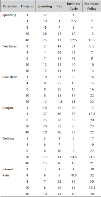
3.4 Forecast error variance decomposition
The fiscal shocks are the strongest short-and medium-term drivers of fluctuations in EA output, besides the business cycle shock. Together, they account for around 60% of the variation in output. Monetary policy shock only plays a larger role in the medium-run.
Turning to the fiscal variables, not unsurprisingly, spending shocks explain the majority of the variation in spending. This is in line with the vision that spending decisions are discrete and therefore less influenced by other economic factors. Variation in taxes, on the other hand, are majorly explained by tax and business cycle shocks. In total these two explain between 80-90% of the variation in taxes over all horizons. Hence, different to spending, for tax decisions, the position in the business cycle at that particular time of the decision matters. In addition, this seems to provide further evidence that the spending and tax policy decisions are taken independently, and are considerate of different factors.
Turning to the monetary side, monetary policy shock explains the majority of the variation in interest rate. Only in the medium-run, does the business cycle shock matter, even if to a limited extent. Again, the position in the cycle matters for monetary policy decisions as far as it provides guidance on the macroeconomic forecast, and thus plays a role in the medium-run.7
Maybe the most interesting aspect of this exercise is to understand the drivers of government debt. While maybe it is not surprising that business cycle shock matters for debt variation over the cycle, a very interesting finding is that monetary policy matters even more for government debt, and its importance increases over the horizon. While in the first quarter after the shock, it explains 16% of the variation (and ranked first), it increases to 22% after the 20th quarter (still ranked first). On the other hand, spending matters little for government debt, and taxes matter more albeit less than monetary policy. This is additional evidence that monetary policy matters for fiscal decisions, via the debt channel, and even more so than the fiscal shocks independently. Interest rate level matters a lot in determining the debt repayment burden, and possibly the reason why it is crucial for explaining the variation in debt level.
3.5 Monetary-Fiscal interactions
My analysis so far has provided firm evidence of monetary-fiscal interactions since 1980's in the EA. Impulse response analyses have shown that central bank reacts to changes in fiscal policy, and vice versa.
However, the reactions are different depending on whether it is a spending-or tax shock. Hence, the monetary authority discriminates between the two policies, as their effects on output are different.Moreover, variance decomposition has shown that monetary policy determines fiscal policy stance insofar that it is determinant for the government debt level and repayment burden, and thus plays a crucial role in determining the budgetary books of the government.
On a deeper level, I find that the nature of monetary-fiscal interactions depends on shocks that hit the economy and the fiscal measure that one considers. If one considers the interaction between spending and monetary policy, then they act as substitutes for the spending, monetary policy, and business cycle shocks. If one considers interaction with taxes, on the other hand, then the two behave as compliments for spending-and business cycle shocks, and as substitutes for a monetary policy shock. However, if one adds the two fiscal policies together and look at the net stance, then for spending and monetary policy shocks, the two behave as substitutes, while for a business cycle shock they act as compliments. For a tax shock, however, the monetary policy does not react and thus I cannot determine any interaction between them.
Lastly, both fiscal and monetary policy react in a stabilizing way to output. However, I find that government spending (contrary to taxes) reacts in a destabilizing fashion to innovations in output since, via the demand-side expansion, it attempts to push output further away from its steady state level. Net stabilization of the fiscal side therefore only occurs because of a larger reaction of taxes than expenditures.
3.6 How important is public debt?
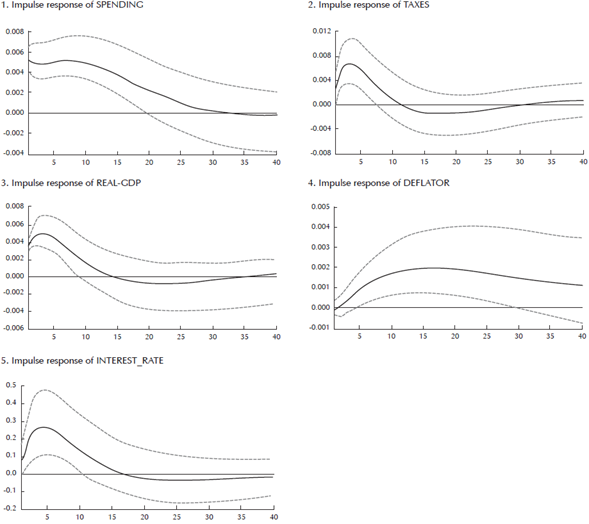
Next, I wish to understand the role that government debt plays in the identification of my model, and the degree to which debt constraints the interactions. There is a widespread view that the three (two fiscal and one monetary) policies affect each other via the impact they have on debt, and thus on the macroeconomy. I wish to validate that view in our model. To do so, I compare our benchmark model to one where I exclude government debt. I then proceed to compare the IRFs, the fiscal multipliers, and the forecast error variance decompositions (FEVD). I need to consider all these estimates since they provide information on different aspects of the model, and thus also the quantitative importance of debt in our bencmark model.
First and foremost, I find clear evidence of omitted variable bias in the estimates when I exclude government debt from our model. Comparing the upper and lower half of Table 4, impulse response estimates in the lower part for variables such as taxes, output or interest rate is different (and mostly higher) than when I control for government debt. Similarly, comparing FEVDs in Table 6 with debt and Table 7 without debt, most of the estimates become upward biased when I exclude debt from the S-BVAR model. In the case of output variation, even the qualitative aspect change when we exclude debt. While for the specification with debt, the three most important shocks for explaining output variation are spending, taxes and business cycle shocks, when we exclude debt in the model, the importance of spending shock dissappears and the majority of variation is explained by tax-and business cycle shocks.
The last exercise compares the fiscal multipliers. As in the previous cases, the multipliers turn much higher when we exclude government debt. However, the difference is even bigger compared to IRFs and FEVDs since the size of the shocks also change. Therefore, the spending multiplier rises from 0.6 in the model with debt to 1 in the model without. Likewise, the tax multiplier rises from 0.125 in the model with debt all the way up to 0.58 in the model without it. The difference is huge. To conclude, our comparative exercises have shown that government debt plays an important role in the identification of monetary-fiscal interactions in our S-BVAR. Failing to recognize the debt channel of fiscal-and monetary policies will result in misinterpretations of the estimates.
3.7 Time-variation
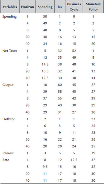
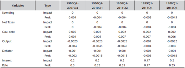
During my sample period, the EA economy went through a number of turbulent episodes and a number of structural changes in policy. In particular, following the subprime crisis and collapse of Lehman brothers, ECB started to engage in unconventional expansionary monetary policy. The fiscal authorities had to bail out many of the banks that were affected by the financial crisis, and many governments engaged in expansionary fiscal policies in order to counteract the contractionary effects from the crisis. Then, following the sovereign debt concerns and the surge in sovereign risk premia for several countries in the EA, the ECB launched its full-blown unconventional monetary package (including the QE from March 2015), and many governments had adopted fiscal austerity measures. In sum, my sample captures periods of both conventional and unconventional monetary policy, and expansionary as well as austere fiscal policy. In order to test whether these policy changes had distinctive structural impacts on the economy, and examine the way in which the two policies jointly responded to these, I will perform an expanding window estimation, augmenting the sample size at each stage with more time-series observations. Table 8 explains the different dates and sample sizes I have selected to estimate.
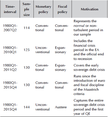
The first period that I estimate is before the onset of the subprime crisis and the beginning of the Great Recession. I consider this period as standard and wish to identify the transmissions and interactions during 'normal' times. The second period includes the first years of the Great Recession, and is just after the date when the ECB officially stated that the EA economies were out of the recessionary region. The third period includes the beginnings of the sovereign debt crisis, when markets started doubting the Greek public finances. Finally, the full sample includes the entire sovereign debt crisis period, and the full-blown unconventional monetary policy artillery. Note that I am not attempting to identify non-conventional monetary policy shocks and determine the effectiveness of unconventional measures. I simply want to see whether the nature of interactions between the two authorities had changed and if the transmission to the real economy had been dramatically altered during this period. For the last subsample, I do not perform an expanding window, but rather wish to test whether the introduction of the Euro in 1999 and the fiscal discipline through Maastricht criteria changed the nature of monetary-fiscal interactions, aligning them more compared to the earlier period.
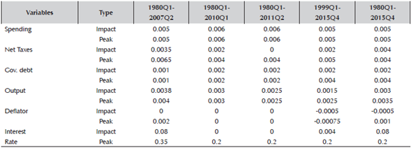
Tables 9 to 11 report coefficients of the IRFs, both on impact and peak. The first thing to note is that many of the IRFs look very similar in the different subsamples. The peak impacts are very close to each other, even if the trajectory of the IRFs throughout the horizon might qualitatively look somewhat different. Hence, the model seems to capture the deep structural links between monetary and fiscal policies in a robust way since they do not vary excessively over different sample lengths. Said that, there are some differences in the magnitudes of the impacts over time.
Table 9: Time-varying estimates for spending shock
Note: Impulse response estimates for a tax shock in different subsamples
Source: author’s calculations.
Table 10: Time-varying estimates for tax shock
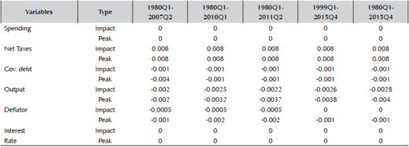
Note: Impulse response estimates for a tax shock in different subsamples
Source: author’s calculations.
Table 11: Time-varying estimates for monetary policy shock
Note: Impulse response estimates for a monetary policy shock in different subsamples.
Source: author’s calculations.
For a spending shock, for instance, the impact on government debt and the variance of the shock was largest during the turbulent period of the financial crisis and the immediate aftermath. For output, net taxes, deflator and interest rate, on the other hand, the largest responses were during the pre-Great Recession (GR) period when the uncertainty in the economy was the lowest.
For a tax shock, on the other hand, the largest response of output, and deflator was during the GR, while that of government debt was before the GR. Lastly, for a monetary policy shock, the largest impact of interest rate movement on spending, net taxes, government debt and output was during the Great Recession, while for interest rate and the deflator, it was in the period before.
Another pattern I found is that the time variation in impact of a shock was the least for taxes. In other words, comparing the three shocks, the least variation in the peak impact we found was for the tax shock. Only three out of the six variables had some time-variation in the peak impact, compared to all six variables for the other two shocks (spending and monetary policy). This is another suggestion that tax shock, different to spending and monetary policy, depends on other indicators such as output and cannot de considered as truly independent policy decision.8
Lastly, one can think that the introduction of the Euro in 1999 and the application of fiscal discipline as a part of the Maastricht package changed the way fiscal policy was conducted, and its interaction with monetary policy. Despite national discretion in fiscal policy setting, the Maastricht fiscal discipline aligned them to an extent and reduced their individual variation. Moreover, the common monetary policy aligned them even further. Therefore, we should expect to see differences in impacts since the introduction of the Euro in 1999. However, our results for the period 1999:I-2015:IV do not differ much to the entire sample period, or the other sub-samples. The peak responses are almost the same as the ones for the full sample. This means that the nature of interactions in EA is deeper and more longer-term beyond a single event. Thus, it is very possible that the process of aligning national fiscal policies was a process that began much earlier, simply consolidating when the common monetary policy was introduced. Thus the interactions we are examining here are of a structural nature spanning over several decades.
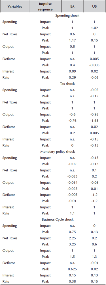
3.8 Comparison to the US
The empirical literature on monetary-fiscal interactions is rather thin, even more so for the EA. In order to put our results for EA into perspective, I wish to compare the estimates with the ones obtained for the US. The results for US are obtained from Gerba and Hauzenberger (2014). I will use the results for the time-invariant S-BVAR model, and the identification scheme for shocks is the same. This in turn allows for a direct comparison between their and our findings. These are reported in Appendix C, Table C.1. The coefficients, labelled as n.s. mean that they are not statistically significant at 95% level.
Table 12 Tax multipliers across the big four in Euro Area
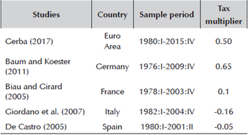
Note: Gerba (2017) study refers to the estimate found in the current paper. All studies, except for Euro Area, do not include the Great Recession period, but that of Germany and France includes the Great Stagflation. In the original studies, the multiplier is defined as an increase in net taxes. However, since in the current paper, we are interested in the economic impact from a reduction in net taxes, at the same time as the models report symmetric multipliers (i.e. the absolute value of the impact from a tax change is the same no matter if taxes are increased or reduced), I have therefore just inverted the sign from the reported values in Kliponen et al. (2015) in order to make them comparable to the EA tax multiplier in this paper.
Source: author’s calculations.
Basically, the impact is clearly different between the two, and these differ depending on the shocks. For EA, the (peak) impact of a spending-and a business cycle shock is beyond doubt more profound, while for the US, it is the (peak) impact of a tax shock. This last finding is very much in line with what we have discussed so far. Tax decisions in the EA are not discretionary and depend on the state of the business cycle. Hence the impact is also limited. In the US, on the other hand, the Congress takes tax decisions and so there is more space for independent manoeuvre. Spending shock, on the other hand, generates a much heavier response of the monetary policy and taxes, and is possibly the reason why spending has a more profound impact in EA. Business cycle swings are also heavier in the case of EA (possibly because there are multiple business cycles within the common EA one), and thus the importance of cyclical swings or the particular position in the business cycle is also wider.
For a monetary policy shock, on the other hand, the difference is not very clear. While the impact on output is more profound in the EA, the reaction of spending and taxes are stronger in the case of the US. Maybe because of this stronger reaction of fiscal policies to a monetary policy shock, the effect on output is milder, and thus why we observe a smaller peak impact.
A comparison of the multipliers in Table 13 shows that while similar for spending, they are very different for taxes. The tax multiplier is much higher in the case of US, with the (peak) impact at 1.65 compared to 0.76 for the EA. That is more than the double. At the same time, while the tax multiplier is higher in the case of the US, it is the spending multiplier in the case of the EA. Hence, in terms of comparative advantages, standard Keynesian expansionary policy seems to be more effective in the EA, and standard non-Keynesian in the case of the US.
To summarize, the impact of shocks is clearly different between the EA and the US, and these differ depending on the shocks. For EA, the (peak) impact of a spending-and a business cycle shock is beyond doubt more profound, while for the US, it is the (peak) impact of a tax shock. For a monetary policy shock, on the other hand, the difference is not very clear. However, the reaction of fiscal policies to a monetary policy shock is stronger in the US. Lastly, in terms of comparative advantages, standard Keynesian expansionary (or spending-oriented) policy seems to be more effective in the EA, and standard non-Keynesian (tax-oriented) in the case of the US.
3.9 Briefly on the tax multiplier across the Area
The number of studies on Europe that specifically incorporate tax multipliers is much scarcer compared to the ones for spending, either because the data on revenues does not stretch sufficiently far back to be used in time-series analyses, data on government revenues are not of good quality or standardized across countries, or because the identification of a tax shock is not as straight forward as for spending. The only available study that includes- and systematically compares tax multipliers across Euro Area is one prepared by the European System of Central Banks (Kilponen et al, 2015) and reported in Table 12. The report summarizes the multipliers found in the VAR literature, so I also report the original references for those studies.
Note that while the multipliers are all extracted from VAR models, the identification methods differ, they do not include a monetary policy shock and the sample periods are not perfectly matching. Therefore while the numbers are clearly comparable and informative, some of the cross-country variation may be due to the aforementioned differences. Said that, this variation should be limited as the economic structure underpinning those multipliers is consistent.
Overall, I find that except for Germany, the other three countries have a lower tax multiplier compared to the Euro Area estimate. At the same time, while that of Germany and France are positive, that of Italy and Spain are negative. For the latter two this might be because the taxes were so low that actually increases in net taxes might lead to a boost in output rather than vice versa, or because increasing taxes for some sectors might improve resource allocation and boost efficiency and, subsequently, output. The first explanation might also, inversely, be valid for Germany, since taxes are already very high there so that a reduction in those will result in a boost in output. Since those estimates do not include the Great Recession period, we might expect that the individual tax multipliers, just as for the overall Euro Area, have increased since the 2007-08 crisis, and opportunities for a tax-led fiscal boost have simply increased.
Compared to the spending multipliers for those individual countries in Table 5, I find the same pattern as for the Euro Area. The spending multiplier is through-and-through higher for all countries compared to the tax one, even for Italy, who has negative multipliers for both spending and taxes. Thus the conclusion that spending increases are more effective in boosting output than tax reductions is universal for Europe and does not only hold for the whole Area, but also for its big four members. Hence, qualitatively the conclusions we draw for the Area as a whole also hold for its biggest members states. That is not surprising since their weights are also proportionally higher in the Area aggregates. Quantitatively, however, we do see heterogeneities amongst the individual countries, which highlights the need to also consider the specificities of each member state when determining the final impact of fiscal policies and the optimal monetary-fiscal mix.
3.10 Robustness checks
To corroborate my findings so far, I perform a series of robustness checks on the benchmark specification for the complete sample. In particular, I test the validity of my previous results by altering the sign restrictions in the identification scheme, by estimating the model in growth rates, and by comparing my findings to results from a plain recursively identified (Cholesky) model. I discuss them in further detail below.
3.10.1 Pure sign restrictions
Arias et al (2014) have shown that in some cases, the penalty function approach might generate biased estimates by adding unintended or unanticipated sign restrictions in the estimation procedure. Thus, the approach might involve additional restrictions on variables that are seemingly unrestricted. To check the consistency of the original estimates, I re-estimate the same model with the same sign restrictions, but substituting simply the penalty method for the rejection method, where all draws that do not satisfy the full identification scheme are discarded. That method is therefore not susceptible to imposing unintended restrictions, and is also less information intensive. The results from this estimation are reported in the third and last segment of Table 4.
In general, the discussion and conclusions regarding interactions from the main text remains. The only difference is that some of the estimates are lower using this method, or that they are not fully significant at the strict 95% interval, but are of a similar size and impact if the confidence interval is relaxed to 80-85%. In terms of individual impulse responses, those of deflator are slightly weaker using the rejection method, while interest rate is slightly less responsive to the other shocks (besides its own). The responses of interest rate are significant at 85% interval. In terms of multipliers, they are in general the same. The conclusion from the benchmark results that the spending multiplier is higher than the tax one remains. The difference is that the spending multiplier is slightly higher when applying rejection method (0,67 compared to 0,60 with penalty method), while tax multiplier is somewhat lower (0,18 compared to 0,50 with penalty method).
To summarize, the conclusions on monetary-fiscal interactions and fiscal multipliers are robust to the estimation method. There is sufficient evidence of interaction between the two policies in an asymmetric manner at the same time as spending increases are more effective in boosting demand and output than tax reductions in the Euro Area even when we use the pure rejection estimation method. The only difference is that magnitudes of some estimates are slightly lower, while spending (tax) multiplier is higher (lower).
3.10.2 Alternative identification scheme
One way to check the consistency of the results discovered in the previous sections is to re-estimate the models but excluding government debt. However, I have already discussed these results and the impact of omitted variable bias on the estimates. I found an upward bias in the estimated impact on output, as well as in the responses in the other fiscal-and monetary policy variables, in particular for the spending shock.
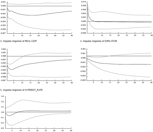
But, another way of validating the results is to estimate the model with the same variables, but alternative sign restrictions. In particular, for the most controversial one, the tax shock, we estimate the tax shock specification removing the sign restriction on debt (i.e. a positive response of tax and a negative response of output, but no restriction on debt).9
I find striking similarity with the results discussed above when I exclude government debt from the model. In this case, I also find that our estimates become biased. In the model without (with) a sign restriction on government debt, the fall in spending and debt is statistically insignificant (significant at -0.005 and -0.002), the fall in output is -0.004 (-0.001), and that of deflator is -0.001 (rise of 0.0005). Hence, by not controlling for the effects of tax policy on debt, the impact on output and inflation are over-estimated, while that of spending and debt underestimated.
Moreover, the fiscal multipliers are very different. In the identification scheme including restrictions on debt, the multiplier is 0.125, while it is 0.57 for the one excluding that restriction. It is clear that the multiplier is overestimated by a factor larger than 4 if the effect of tax changes on debt are not taken into account.
Thus, the fiscal policy-debt channel is very important to include if one wishes to obtain unbiased estimates. An important conclusion from this exercise is that not only do we need to consider monetary policy when we estimate the effects of fiscal policy, but we also need to include debt and provide a rationale for debt dynamics if we wish to obtain a complete and unbiased picture of the effects of fiscal policies.
3.10.3 Estimation in growth rates
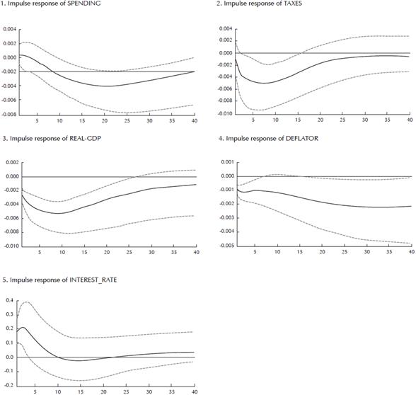
To check the robustness of my benchmark results, I performed the sign-restriction estimation with data expressed in annual growth rates. The unit root tests showed that my data have a I(1) process. Thus, following the hotly debated topic of whether SVAR models with I(1) data should be estimated in levels or growth rates, we re-estimated our model in Section 4.1 but with all variables expressed in annual growth rates (except for the interest rate). The estimation procedure is still based on the penalty function method and we use the complete sample period from 1980Q1-2015Q4.10 Both the qualitative and the quantitative results remain.
Following a positive spending shock (of 0.75%), taxes increase in order to finance some of the spending rise, however only at 0.5%. As a result, government debt increases by 0.4% and remains persistently above the trend for almost 40 quarters. The fiscal expansion results in a GDP increase of 0.30%, and an inflation of 0.1%. As a reaction to this expansion, interest rate increases by 0.4%, which considerably above the rise in inflation.
I find a very similar evolution for a tax shock as in the benchmark model. A monetary policy shock of 0.1% has significant impact on taxes. They fall by 0.65%, while spending remains more or less unchanged. The tax-based fiscal expansion results in a government debt expansion of 0.4%. At the same time and following the interest rate increase, inflation falls immediately by almost 0.3%, and output by 0.4%.
To end and following a business cycle shock (0.8% increase in output), taxes rise by 1.5% (as the tax base has increased) and spending rises by 0.4%. Since the rise in taxes is higher than that of spending, the net fiscal effect is contractionary. That is why government debt falls (by 0.6%). Faced with a rising inflation (0.15%), the monetary authority tightens their policy by increasing the policy rate by 0.5%.
To finish, my original findings remain when I estimate the model in growth rates instead of levels. Hence, the method is robust to the data specification in the model.
3.10.4 Comparison to a recursive scheme
The last robustness check concerns the way I identify the shocks. To validate the robustness of my benchmark results, I re-estimate the same model but identify shocks based on a simple agnostic Cholesky identification approach. Hence, I use the same Bayesian estimation procedure and set lag equal to 2 for the endogenous variables. I also use a Normal-Wishart prior and correct for the degrees of freedom as in the previous section. Lastly the order of the variables entering the model is the same as before (spending first, followed by taxes, government debt, output, deflator, and interest rate last).11
Using the recursive scheme, the identification of the model is much weaker. Most of the IRFs are not statistically different from zero (except for the shocks). Second, even in the cases where they are, the magnitudes of the response-variables are much smaller. The only similarity I find with the previous identification procedure is that the link between taxes and interest rate remains. Following a tax shock, interest rate rises by 0.2%, and following a monetary policy shock, taxes rise by 0.006%. In contrast, the link between spending and interest rate dissappears. Interest rate does not respond to spending shocks, and vice versa. That is not the case in the sign-restriction version of the model, where the link between spending and interest rate is tight.
To conclude, this exercise shows that the structural identification scheme consisting of sign restrictions is strictly superior to the simple Cholesky decomposition. The identification is more robust, the impact of shocks stronger, and the interpretation of the impulse responses is structural and with theoretical foundations. All in all, all the robustness exercises show that the method and identification scheme applied in the paper is robust and consistent with the underlying economic theory.
4 Conclusion
The joint analysis of monetary and fiscal policy in the EA sheds novel light on the role and effects of (common) fiscal policy and their interactions with monetary policy since 1980. I find sufficient evidence for a common fiscal policy reaction in the EA, both in terms of (endogenous) impulse responses and shock decompositions. I also find significant evidence for (implicit) interactions between fiscal-and monetary authorities. Said that, the nature of interactions depends very much on the shocks that hit the economy. While for a spending and monetary policy shock they act as substitutes, they act as compliments for a business cycle shock. At the same time, the way the two fiscal policies interact with monetary policy is also different and independent of each other. On the effectiveness of fiscal policies, I find that the spending multiplier is higher than the tax multiplier. Nonetheless, this efficacy has changed over time, and while the spending multiplier has decreased since the onset of the Great Recession, that of taxes has increased. I also show that it is crucial to include government debt in the estimation of monetary-fiscal interactions. Failing to recognize the debt channel will result in misinterpretation of the monetary-fiscal estimates. To conclude, there are considerable differences in the nature of monetary-fiscal interactions between the EA and the US. Not only are the impulse responses to different shocks significantly different between the two economies, but also the fiscal multipliers vary a lot. Standard Keynesian (or spending-oriented) fiscal policy is more effective in expanding output in the Euro Area while tax reductions are more effective in the US.
Even if this is one of the first attempts to structurally understand the joint behaviour of fiscal-and monetary policy in the EA, there are multiple ways in which this analysis can be improved and extended. Recognizing that the EA economies have undergone significant structural changes since 1980, it would be purposeful to estimate the interactions within a time-varying parameter VAR, as Gerba and Hauzenberger (2014) have done for the US. Another interesting extension would be to estimate the interactions using a strategic interactions set-up based on theoretical models on monetary-fiscal interactions (such as e.g. Leeper (1991) or Davig and Leeper (2011) to determine leaders and followers in policy setting. Alternatively, one could cast these policies in a jointly estimated model for EA member states and the EA as a whole (possibly in a G-VAR). This would permit to investigate the level of fiscal spillovers in the monetary union, and whether having a common monetary policy has lead to an alignment in fiscal policies across the union. This would allow for a formal test of the policy spillover hypothesis initially proposed as a part of the extended OCA theory.