English (pdf)
 Article in xml format
 Article references
 Send this article by e-mail
 Cited by SciELO
  Cited by Google
  Similars in
SciELO
Similars in
SciELO  Similars in Google
 Permalink
Introduction
In any country, the government plays an important role in economic dynamics. The government’s decisions have an important impact on the other economic agents (consumers and firms) in terms of income, consumption, and investment. This becomes even more important in developing economies since they present significant challenges to fulfill the main functions of fiscal policy. The degree of economic openness, access to credit, debt interest payments, pension management, and corruption are only some of the factors that hinder the fulfillment of the three main functions of fiscal policy1. These factors affect the ability to solve structural problems and maintain a degree of flexibility according to countercyclical policies (Buti et al., 1998). Fiscal policy also affects long-term growth through capital accumulation, debt level, debt rating, the crowding out effect and externalities produced by public expenditure, and the quality of public policies implemented.
In addition, it is important to note that there is a close relationship between the business cycle and fiscal policy result. In the cycle expansion phase, the levels of investment, consumption, output, employment, and profits of companies increase. This triggers a greater dynamism of tax collection, and, assuming that expenses do not increase in the same way, bring about a better fiscal balance. In the contraction phase, the opposite occurs and a fall in economic activity and tax revenues ensues, which translates into imbalance in government finances. Thus, a fraction of the fiscal balance has a cyclical component, determined endogenously with the behavior of the economy, and that does not depend on the discretionary management of fiscal policy.
The factors mentioned above not only justify the importance of the workability of fiscal policy, but also create the need to quantify the fiscal policy in order to provide information about its impact when performing an intervention. In the literature, this measure has been denominated as fiscal multipliers (public expenditure and tax revenue). While there are a large number of studies on multipliers, there is no consensus on their size, which generally differs among countries. A large review of the size of fiscal multipliers can be found in Baunsgaard et al. (2014) and in Mineshima et al. (2014). The latter review forty-one studies using VAR and DSGE models, both linear approaches. They find that the expenditure multiplier ranges from 0 to 2.1 with an average of 0.8, while the tax revenue multiplier ranges between -1.5 and 1.4 with an average of 0.3.
However, recent literature has focused on analyzing the relationship between fiscal multipliers in light of the state of the economy. Authors such as Baum et al. (2012) find that the cycle's position affects the impact of fiscal policy on the G7 economies, and show that average tax and expenditure multipliers tend to be larger in periods of recession that in periods of expansion.
In Colombia, few studies have been made on fiscal multipliers, hence the importance of addressing the issue especially to understand the dynamic effects on economic activity. For this work, considering the existence of a cyclical fiscal component, we believe that treating the quantification of the multipliers and the relationship between fiscal policy and growth in a linear manner is not the most appropriate choice, considering that, among other things, the transmission mechanisms are complex. Therefore, we calculate the impact of these multipliers depending on the position of the economic cycle, e.g., non-linear multipliers of public expenditure and tax revenue, an aspect that has not been studied in the literature so far. To fulfill this objective, we implemented a methodology that allowed for the study of magnitude and sign, given the potential non-linear effects that could take place according to the state of the economy defined by the output gap, positive or negative. For this purpose, we used a Bayesian estimation of a non-linear multivariate time-series model, in this case, a Logistic Smooth Transition VAR model (Bayesian LST-VAR). Using this methodology, this research seeks to answer questions such as the following: Are the multipliers of public expenditure and tax revenue state dependent? Are they greater in magnitude in times of low economic growth or in times of greater growth? Which of the two multipliers has the highest impact on growth?
Based on the above and with the aim of answering the research questions, this document provides the context of the period studied. After that, it presents a review of concepts and literature related to fiscal multipliers and business cycles. Then, it explains the methodology for linear and non-linear analysis. Finally, it shows the results and conclusions of this research.
1. Historical context of the period under study
Before starting with the technical and theoretical part of the work, we believe it is important to briefly describe the historical context and the economic conditions of the period under study, which covers from 1994 to 2015. To do this, we will concentrate on analyzing the most relevant facts considering changes and fiscal transformations in order to present a broad framework to provide ideas on the structural fiscal balance, decentralization, the General System of Royalties (GSR) and the General System of Participation (GSP).
First of all, it must be said that the size of the state has increased. According to Gómez and Posada (2002), the level of public expenditure was modest in Colombia until the end of the 1970s and began to increase significantly only between 1980 and 2000. This caused public expenditure to increase from about 9.0% to more than 33% of Gross Domestic Product (GDP), not including public debt service. In that period, public expenditure was transformed mainly into investment in human capital (health and education) and infrastructure.
Within this process of state size transformation, some changes took place. One of the most important was the decentralization process, which began mainly in 1980 and was consolidated with the 1991 political constitution. The purpose of this process was to strengthen regional finances in order to provide fiscal autonomy to municipalities and departments. This was materialized with the implementation of different laws2, where the tax on liquor, cigarettes, and gasoline was changed at departmental level, while at municipal level some changed was about the cadastral appraisals for the property tax and the assignment of rents were carried out value-added tax (VAT). With the Colombian constitution of 1991, decentralization (not only fiscal but also political) was deepened. New parameters were established for fiscal assignment towards the departments, and there was an increasing participation of the municipalities in the current revenues of the nation and the rights on royalties. Subsequently, the transfer of resources and competences was regulated. Finally, in 2012, royalties were regulated, thus ending the process of decentralization, broadly speaking.
This shows that the decentralization process has been a transfer of resources and responsibilities from the national administration to the subnational ones. This triggered a greater size of the state with regard to institutions and staff, in order to respond to these responsibilities in the territorial entities. In order to do so, in addition to expenditure on education, health, and infrastructure, increased social expenditure, justice, security and other administrative expenses were raised. However, problems of adaptation and workability in the implementation have reflected failures of the fiscal environment from different origins. For instance, problems with tax collection and generation of resources. Additionally, there were issues on budget execution (on the expenditure side) due to legislative reasons such as tax rigidities. Reflecting this, but not necessarily causing it, a progressive deterioration in the territorial and central government finances took place since 1992. Between 1990 and 1999, the territorial fiscal deficit went from 0.3% to 0.6% as a percentage of GDP, and there was a central government deficit from 1.0% of GDP to 6.8%.
It should be noted that the transfers to the municipalities and departments from the decentralization process generated important fiscal effects and in macroeconomic terms. Junguito et al. (1995), considering the period from 1967 to 1994, found that transfers caused greater fiscal effort, translated into growth in tax revenues of municipalities and departments, contradicting the thought of fiscal laziness. Nevertheless, they also found that by increasing transfers by 1.0%, the central government deficit increased by 1.04%. Thus, territorial finances can affect the consolidated public deficit by means of balance sheets, regional indebtedness, or mismanagement of resources, for instance. Recently, Julio and Lozano (2015) also confirmed a positive relationship between fiscal decentralization and economic growth in all regions of Colombia based on two income indicators and two expenditure indicators.
Given this deterioration, some studies tried to identify the determinants of the evolution of the same for the central national government mentioned above. Lozano and Melo (1996) focus on the fiscal deficit of the non-financial public sector. They show that between 1985 and 1996, the deficit was determined by national government operations, since in most years the decentralized entities offset the imbalances. In their analysis, they identify three periods. First, adjustment; second, stability; and third, from 1992 to 1996, the period of deterioration, where decentralization and the strengthening of new entities materialized in the expansion of expenditure together with the payment of debt interest. These were the main determinants of deepening the unbalance in a context where fiscal policy was pro-cyclical until 1998 and counter-cyclical for the next four years.
The situation of the Central National Government (CNG) is not very different, given that the evolution of expenditure places it near 19%, showing an 11% increase as a percentage of GDP between 1990 and 2016. It is worth noting that, as mentioned by different studies such as Toro and Lozano (2007), the existing deficit has been of a structural and non-cyclical nature, pointing out that for 2006 only 17% of the fiscal imbalance was related to the cyclical component. Lozano et al. (2013) point out that on average, only 10% of the fiscal imbalance registered by the Non-financial Public Sector (NFPS) between the end of the 1990s and the beginning of the 2000s is due to the low growth of economy, reaffirming the problems rooted in the Colombian fiscal structure.
When analyzing territorial finances (table 1), it is observed that in recent years, transfers from the SGP and the SGR have had significant shares of income. Both represent about 55% of the total income, evidencing a high degree of dependence of the municipalities and departments. In particular, income from royalties has an average growth rate of 12%, while that from tax revenues is 2.0%. There has been variation in the tax measures implemented, in particular, the most recent tax reform of 2016. In general, a greater institutional effort should be made to increase collection and reduce issues such as evasion in many operations. Additional work has been done on issues of labor formalization and banking for instance in the commercial sector, where many cash transactions provide secrecy and tax evasion. Investment accounted for 82% of expenditure, exhibiting significant growth over the last three years. The average result shows a total deficit of 0.12% and current surplus savings closing 2015 at 2.4%, both as a percentage of GDP.
Table 1 Financial Aggregates of the Central Municipal and Departmental Governments as a % of GDP
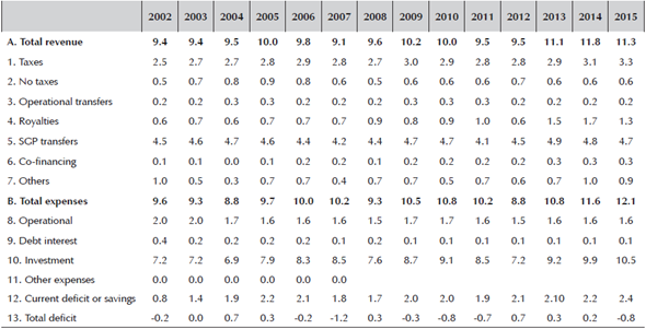
Source: Adapted from the National Planning Department (DNP).
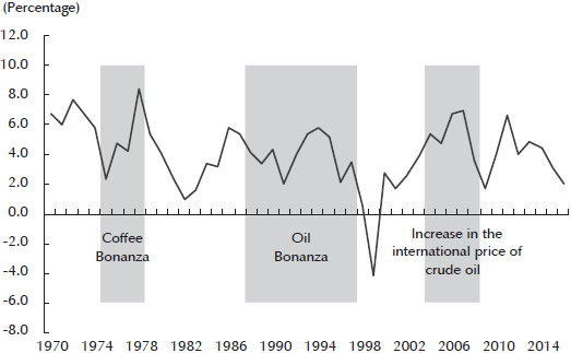
Other important macroeconomic aspects that have affected the government’s public finances have been the management of external bonanzas (coffee in 1977, oil in 1987, and the recent “commodity boom” in 2002), which may deepen or dampen the economic cycle. Colombia has not had the best experiences in managing bonanzas. Thus, Colombia has shown the need to adopt public policies to save surpluses from bonanzas because, in general and beyond the economic cycle, the periods of abundance have been followed by recessions, loss of international reserves, depreciation, unemployment, and bankruptcy of companies, as happened after the coffee boom (Figure 1). All of those, in addition to sharp declines in public savings from 8.0% of GDP to a level of depletion of 0.2% of GDP between 1995 and 1997, occurred after the first oil boom (Minminas, 2011). This last fact, added to the high levels of indebtedness of the country, generated restrictions to respond to the financial crisis of 1999.
Although an external bonanza is not part of the economic cycle because it is characterized by unexpected shocks in prices or production, the management of the resources obtained from them by the authority can deepen booms or recessions, considering the spillovers on the level of indebtedness, the degree of economic openness, the exchange rate, and the crowding out effect in factors of production from tradable to non-tradable goods by increasing relative prices (Ismail, 2010). It is here that fiscal policy maker plays an important role in how to manage the resources to stimulate the aggregate demand and employment in times of recession as well as in periods of expansion.
This information sought to provide a general context of the country's fiscal outlook, given that the figures from the CNG and the NFPS show significant fluctuations from different origins over the last decades. Decentralization and transfers from the government to territorial entities, the economic cycle, oil price fluctuations, and some regulatory and legal issues, among other factors, have been mainly responsible for these variations, which can influence directly or indirectly the change in the size of the multipliers.
2. Fiscal Multipliers and Economic Cycles: Concepts and Literature
It is important to start with the definition of a fiscal multiplier. In line with Spilimbergo et al. (2009), a fiscal multiplier measures the change on product due to an exogenous change in the fiscal deficit with respect to a baseline. Depending on the purpose, different types of tax revenue multipliers can be calculated. In this particular case, we will focus on:
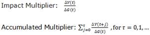
where G represents Expenditure or Tax Revenues.
This paper seeks to quantify the effect produced by the change in any of the two fiscal variables; public expenditure or tax revenue. The impact multiplier will measure the amount in which the product varies when expenditure or taxation changes by 1.0%. On the other hand, the accumulated multiplier (e.g., for expenditure) will measure the accumulated change in output per unit of additional expenditure from the moment of the impulse to the desired horizon.
In addition to the importance of quantifying the effect of fiscal policy on output, multipliers have an impact on designing policies. Eyraud and Weber (2012) point out that underestimation of these multipliers may lead countries to set unreachable targets, failing to calculate measures such as the necessary adjustment in the debt ratio. These constant failures may affect the trustworthiness of fiscal government consolidation programs.
The resulting multipliers tend to be heterogeneous across countries. In general, the size of the multiplier is conditioned by idiosyncratic variables of each economy. Hemming et al. (2002) present a comprehensive literature review, theoretical as well as empirical. They explain various influences on the multiplier effects of government expenditure increases and tax cuts. For the demand side, they describe effects associated with the Keynesian approach and crowding-out in an IS-LM framework. They also analyze non-Keynesian effects such as rational expectations, Ricardian equivalence, consumption smoothing, interest rate premium, and credibility. They analyze the supply side and institutional aspects, with the latter being the most important because, in addition to management responsibility, institutional factors are important for inside and outside lags in the workability of the fiscal policy.
In this regard, Ilzetzki et al. (2013) use a SVAR to indicate some generalities found for forty-four countries in the behavior of the multipliers according to some specific characteristics of the economy, as follows:
In developing countries, output increases in response to a shock in public consumption with a delay (2-4 quarters). In these countries, the effect of fiscal policy falls deeply and the multiplier is smaller, while in high-income countries the effect is persistent (Estevão and Samake, 2013).
Flexible exchange-rate economies tend to have smaller multipliers than economies with a fixed exchange rate, in line with Born et al. (2013).
Trade openness degree matters: relatively closed economies have multipliers between 1.3 and 1.4. .The multipliers tends to be larger in more opened economies, because the shock effects extended to other countries through the import channel which do not operate with the same strength in closed economies-
Two final features are a high level of debt (Ghosh & Rahman, 2008), and large size in automatic stabilizers make the multipliers smaller (Dolls et al., 2012).
However, a large number of studies such as the previous, despite being rich in the number of countries analyzed and in data availability, do not consider that multipliers can change because of the idiosyncratic characteristics of each economy, but also depending on the business cycle. The understanding of this last phenomenon is tied to a great diversity of literature such as the classical ((Mitchel (1927), and Burns &Mitchel (1946) and on growth (Lucas (1977), and Kydlan & Prescott (1990)), among other research such as Blinder & Fischer (1981) or Hamilton (2011). In general, all show the fact that, at certain times, the economic activity is stronger than in others, and it is diverse in terms of breadth and duration.
For the empirical analysis of economic cycles, linear approaches have been widely used. However, since Mitchell (1927) and Keynes (1937), there is evidence that economic contractions are shorter, more volatile, and more violent than expansions, and that the underlying series exhibit non-linear behavior. Hence the need to incorporate this non-linearity in macroeconomic modeling. Authors such as Hamilton (1989), Teräsvirta & Anderson (1992), Granger & Teräsvirta (1993), Potter (1995), Hansen (1997), and Tsay (1998), among others, have formalized and have been pioneers in modeling these dynamics with Markovian switching models (MS), smooth transition (STAR), or threshold (TAR) regression models.
Although this work does not seek to explain the causes of economic cycles, it is framed under a non-linear methodology for different reasons. The first reason is associated with the presence of expansion and recession phases in the study period, e.g., the non-linear effect of the economic cycle. The second reason is associated to the non-linearity that can produce the fiscal variables such as the following. In the case of expenditure, when the economy is in recession, effects such as crowding out are attenuated given that there is excess of installed capacity, so the multiplier effect on aggregate demand may be different in expansion than in recession. On the tax side, when the economy is expanding, tax revenues associated with consumption tend to be higher than when the economy is in recession, affecting not only the fiscal balance policy, but also public policies, which can be made with that type of income.
These ideas can be collected in three types of potential non-linearities, which confirm that the non-linear treatment is the most appropriate. The first non-linearity is associated with the impact of the multiplier according to the state of the economy, e.g., if public spending is increased by 1.0%, the response of the fiscal multiplier may be higher or lower depending on the economic conditions of a particular country (GDP growing above or below potential GDP). The second non-linearity, or asymmetry as other authors call it, is associated with the sign of the shock, e.g., if the 1.0% increase in expenditure produces a 1.1% increase in GDP, a reduction of 1.0% will not necessarily translate into a 1.1% reduction of GDP. The third factor of non-linearity is associated with the size of the shock, that is to say, if the 1.0% increase in expenditure produces a GDP increase of 1.1%, a 10% increase will not necessarily produce a GDP increase of 11%.
Meanwhile, isolating the effect of fiscal policy has become an empirical challenge: there are several studies and techniques available to calculate multipliers. A review is then made using linear and non-linear methodologies.
In their seminal paper, Blanchard and Perotti (2002) implement a SVAR framework with quarterly data for the USA. They found that a positive shock in expenditure has a positive effect on GDP, and that a positive shock in taxes has a negative effect on gross domestic product. The size of the multiplier is relatively small. Among other studies for the United States are the following; Fatas and Mihov (2001), who find that the response of economic activity to changes in fiscal policy is strong, positive, and persistent. They point out that taxes, transfers, and government employment are the most effective tools of fiscal policy. Canova and Pappa (2007) consider the relationship between local fiscal policy and price differentials in monetary unions. They consider two types of expenditure shocks and one type of revenue shock; also, they use sign restriction on the responses of output and deficit, and suggest that fiscal policy is a modest but statistically significant source of price differentials. For other interesting studies related to these, see Canzoneri et al. (2002), Mounford & Uhlig (2002), and Galí &Perotti (2003).
For industrialized countries, several studies have been carried out. In the euro area, Burriel et al. (2010) use the framework in Blanchard and Perotti (2002) to study the impact of aggregated and disaggregated government expenditure and net tax shocks. They explore the sensitivity of including variables aimed at measuring “financial stress” (increases in risk) and “fiscal stress” (sustainability concerns). In addition, De Castro & de Cos (2006) for Spain, Heppke-Falk et al. (2010) for Germany, and Giordano et al. (2007) for Italy, complement some studies.
In an emerging market economy, it is unclear whether the multiplier should be higher or lower because there are factors on both sides. Some studies for emerging market economies are Tang et al. (2010) for Malaysia, Thailand, Singapore, and Philippines.
As for Latin America, the empirical literature is not vast. Restrepo and Rincón (2006) use SVAR to calculate the multiplier for Colombia and Chile. They find that in the case of Chile, a tax revenue multiplier reduces GDP to 0.4, while the expenditure multiplier is 1.9. In Colombia, the tax multiplier is statistically null, and in the expenditure case, the multiplier is 0.15. Céspedes et al. (2013) conducted research for Chile examining the non-Ricardian effects of government expenditure shocks and confronting the evidence of the VAR model with the forecast from a DSGE model. Sánchez and Galindo (2013) find an expenditure impact multiplier of 1.2 for the Peruvian economy, while the accumulated multiplier is 2.2. On the tax side, the impact multiplier is 0.2 and null in long-term horizon. Finally, Estevao & Samake (2013) conducted research for Central American countries. They found that the impact multipliers for total expenditure is between 0.01 and 0.44 and the cumulative multipliers for total expenditure between 0.45 and 0.94.
The discussion on the role of fiscal policy in economic activity takes a deep interest particularly when economies enter into periods of recession. Blanchard and Leigh (2013) investigated the relationship between growth forecast errors and fiscal policy in the crisis period of 2009. They found that the fiscal multiplier was greater than forecasted for this period. This conclusion is supported by Fatás & Summers (2015), in line with the idea that in times of crisis, or at least where there is a negative gap in GDP, the multiplier was greater. The latest research gives way to non-linear models through the literature, whose research indicates asymmetric effects in the multipliers.
Auerbach & Gorodnichenko (2012, 2013) conducted two studies on fiscal multipliers. In their first paper, the authors use a STVAR to provide the transition of an economic state to others and then calculate the multipliers. For both regimes, they show an impact on GDP close to 0.5. However, the impulse response function (IRF) shows that in times of upturn, the multiplier effect falls quickly, while in slump periods the effect is permanent and reaches a peak close to 2.5 after 20 quarters. In the second paper, the authors adapt their previous methodology and use direct projections rather than the SVAR approach to estimate multipliers for OECD countries. They find that GDP multipliers of government purchases are larger in a recession.
Baum et al. (2012) analyze six G7 countries, while Afonso et al. (2011) analyze four countries. They use threshold VAR models and TVAR for a shift in the economy state. Both papers show that, on average, both multipliers are bigger in times of downturn than in expansion. Likewise, Batini et al. (2012), using a non-linear methodology, provide a similar analysis for the United States, Japan, Italy, and France. Among other research that have also used non-linear methodologies, Bachmann and Sims (2011) for the United States and Baum and Koester (2011) for Germany stand out.
In Latin American countries, Sanchez and Galindo (2013) found an asymmetric multiplier for Peru using a LSTVAR. They show that an expenditure multiplier is greater than a tax revenue multiplier, and that both are greater in downturns than in expansion. The multiplier tax when the output gap is negative ranges from 0.1 to 0.25, while the expenditure multiplier range is from 1.25 to 1.35.
In the case of Colombia, in addition to Restrepo & Rincon (2006), it is important to highlight the DSGE model, FISCO, developed by Rincón et al. (2014). The main predictions of this research are: positive and transitory shock to tax rate; decreased GDP, consumption, employment, real wages, and inflation; improvement of the fiscal balance and debt indicator. On the other hand, the positive shock to the operating expenditure raises GDP, consumption, employment, real wages, and inflation. In turn, it raises the interest rate and reduces investment, and worsens the government balance sheet. They analyze a positive shock to oil revenue and find that GDP and consumption rise, but that employment, real wages, and private investment reduce, exchange rates appreciate, and private exports deteriorate, while the government’s balance sheet improves and debt is reduced. As for the size of the multipliers, they find that the tax revenue multiplier is small, around -0.2. The expenditure multiplier is greater than taxes and its sign changes depending on whether the increase in expenditure is financed by a cut in operation or investment. In the first case, the impact multiplier is 0.3, while in the second it is -0.1. Finally, López (2016) shows that the balance sheet effects might reduce the fiscal multiplier by half, developing a DSGE model à laBernanke et al. (1999) with financial friction and non-Ricardian households. Vargas et al. (2013) use non-linear models, although they do not calculate tax multipliers.
As far as the exploration of asymmetries, the study by Lozano et al. (2009) stands out. They use TAR and MTAR models to assess whether the process of adjusting income and expenditure is symmetrical. However, they do not find evidence in favor of asymmetries, although their analysis is not oriented to the calculation of multipliers.
Another methodology frequently used to measure fiscal shocks is the narrative approach. This approach seeks to identify exogenous fiscal shocks directly. More information can be found in Romer and Romer (2010), Favero & Giavazzi (2012), and Cloyne (2013). However, it is not of interest for this work.
3. Methodology
As stated by Blanchard and Perotti (2002), at least two reasons support the structural VAR approach. “First, budget variables move for many reasons, of which output stabilization is rarely predominant; in other words, there are exogenous (with respect to output) fiscal shocks.” … Second, “… decision and implementation lags in fiscal policy imply that, at a high enough frequency-say, within a quarter-there is little or no discretionary response of fiscal policy to unexpected contemporaneous movements in activity. Thus, one can construct estimates of the automatic effects of unexpected movements on the activity on fiscal variables, and, by implication, obtain estimates of fiscal policy shocks. Having identified these shocks, one can then trace their dynamic effects on GDP.” This is how it is done in this paper.3 We obtain the non-linear impulse response, in the sense of Bruns & Piffer (2016) or generalized IRF, which are not prone to ordering.
In order to study the impact of policy on the transmission of fiscal shocks, we estimate a Smooth Transition Vector-Autoregressive (STVAR) model with two exogenous regimes. Particularly, we use a logistic transition function. The two regimes are defined with respect to the level of our GDP-gap (positive or negative expansion or contraction). It is worth mentioning that logistic transition function was always favored against exponential specification, as shown below.
The eight-variable STVAR includes GDP growth, Taxes, Government Expenditure, Terms of Trade, Openness degree (as Export plus Import as a proportion of GDP), U.S. Federal Funds rate, Interbank Interest Rate, and Government Debt to GDP ratio.
The system can be written as:
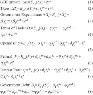
Expenditure and tax shocks are pulled out from their own perturbation. This corresponds to a 1.0% shock as, was stated in the introduction. Thus, 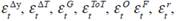 and
and  are the structural innovations to demand, taxes, government expenditure, terms of trade, openness, foreign, interest rate, and debt shocks, respectively. These shocks are assumed as contemporaneous, independent, and uncorrelated with every variable in the information set and with any other shock. In other words, they are assumed to be rational expectation errors. It is also understood that they are contemporaneously independent and uncorrelated.
  refers to the mathematical expectation of the respective conditional variable on all the information available and observable variables at time t-1, including past data.
The conditional expectations given in equations (1) to (8) are replaced by lag projections of the variables in the system. Hence, they can be expressed as a VAR system where the vector of variables summarizing this is  with a with a vector of structural shocks given by
5. Data, Model, and Estimation Approach
5.1 Data
We used quarterly data from Colombia from the period between 1995Q1 and 2015Q4. The variables used were real Gross Domestic Product, tax revenue, public expenditure, terms-of-trade index, openness degree, the U.S federal funds rate, the interbank interest rate (IBR), and the debt-to-GDP ratio. According to the literature, the last five variables are exogenous, but are characteristic to the Colombian economy. Finally, the variable we use to represent the state of the economy is the output gap, which is obtained with the Hodrick-Prescott filter. However, six other gap indicators were tried, all showing similar results to those presented here.4
We worked with data from the Central National Government (GNC) and chose tax revenue and public expenditure variables. Regarding the public expenditure variable, we chose investment and operating expense. For the tax revenue variable, we added income taxes, internal and external VAT, and the tax on financial movements, among others. This variable was chosen from the data available; emphasizing that there may be limitations in the analysis due to changes in the tax base or tax rates.
The sources of the series used were the Central Bank of Colombia, Ministry of Economy and Finance of Colombia, DANE, and the Federal Reserve Economic Data. Fiscal variables were deflated using the CPI (Consumer Price Index), and, additionally, all the series were seasonally adjusted using the TRAMO SEATS methodology. All the series are stationary after suitable transformations, as indicated by the unit root tests previously performed.
5.2. The Model: A Non-linear Smooth Transition VAR Model
The only transition variable we used was the output gap. The reasons to employ the output gap in line with Baum et al (2012) are manifold. The output gap is the most commonly used measure to identify economic cycles, because it is considered not only as reliable ex-post, but also as a reliable real-time indicator for policy-makers.
The estimations of non-linear IRF on GDP from a unit shock to T or E start from the model along the sequence given by equations (1) to (8) in section 4. This model will be specified as a smooth transition VAR (LST-VAR) model,5 which allows us to model and diagnose the types of endogeneity and non-linearity of fiscal multipliers (FM) discussed above. Two alternative specifications were tried: logistic and exponential.6 The models are estimated and selected by Bayesian methods, following closely the approach implemented by Gefang and Strachan (2010), and Gefang (2012), and by the use of Bayes Factor as described below.
The Bayesian approach has several advantages. The multivariate estimations of linear and non-linear smooth transition models are rich in parameters, so inferences can be very sensitive to model specifications such as lag order. Optimization algorithms of the likelihood functions can be unstable, and prediction and understanding of dynamics depend on asymptotically justified methods such as the bootstrap (Koop & Potter, 1999). Likewise, Fernandez-Villaverde (2010) lists additional justifications to use Bayesian methods in economic and econometric analyses. The advantage of this paper is that it implements a Bayesian approach for estimation, inference, and prediction, which allows us to perform a joint estimation of all model parameters, avoiding grid-search type of procedures which may generate unstable estimations. Movements of the endogenous variables will depend on their own lags and on the different shocks. Moreover, regime changes are determined by the transition variables, whose dynamic is captured by a logistic smooth transition function. The p-lags order LST-VAR model is written as (see He et al., 2009):

With A(L) and B(L) being p-order polynomial matrices; L being the lag operator;  being a diagonal matrix whose elements fj are transition functions, with
  representing the cumulative function of logistical probability for the transition variable, zt the output GAP, and γ the smoothing parameter for the change in the value of the logistic function (γ >0). Thus, the smoothness of the transition from one regime to the other has the following behavior: if γ is very large, the logistic function
  approaches the indicator function I(zt > 0). As a consequence, changes from 0 to 1 become instantaneous at zt=c. When γ approaches zero, the logistic function becomes a constant (equal to 0.5) and the LST-VAR model reduces to a linear VAR model with parameters
 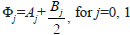 , …, p.
On the other hand, c is the localization parameter and can be interpreted as the threshold between the two regimes in the sense that the logistic function fj(·) changes monotonically from 0 to 1 as zt increases. Finally, μt is a vector of white-noise processes. Parameters γ and c together with zt govern the transition between regimes. Thus, when γ → ∞ and zt < c, we are under the regime of A(L)Yt-1, while when γ → ∞ and zt > c, we are then under [A(L) + B(L)]Yt-1. For finite values of γ, one has a continuum between the two extreme regimes.
The structural shocks in equation (9) are identified by using the Cholesky decomposition. In other words, we define μt = A-1εt, with A being an inferior triangular matrix and ε the vector of the structural shocks, which are assumed to have the following properties:  not cross-correlated and
The Cholesky decomposition ordering is chosen because it does not affect the robustness of our estimates since they are constructed using GIRFs, which are quite robust to the ordering of the variables in VAR systems (Pesaran & Shin, 1998; Ewing, 2001). Second, innovative work in the field of Bayesian non-linear VARs (such as Gefang and Strachan, 2010; Gefang, 2012) considers that the Cholesky decomposition is a good approximation of identification, which is complemented with GIRFs to overcome the issue of ordering the variables in a VAR system. Therefore, the critiques by Faust and Rogers (2003) stating that we are using a recursive identification method do not hold for our estimations.
One possibility to select the p-order of the system, to choose the transition variables z, and to know the lag delay d of the transition variables and the values of the parameters γ and 𝑐 is to have a range of models and then choose the best one using, for example, the maximization of the likelihood function as a criterion. This is commonly done by the applied literature on non-linear models, for instance by Winkelried (2003), González et al. (2010), and Mendoza (2012), who use data from Latin American small open economies.
An alternative, as chosen for this paper, is to use Bayesian methods to formally compare specifications among different models (remember that under the Bayesian approach models become random variables). Specifically, we calculate the Bayes factor from the Savage-Dickey density ratios (SDDR) for many combinations of the arguments and compute posterior model probabilities to select the dominant model for inference.7 This allows us to account for model specification and coefficient uncertainties, as well as for the driving forces of the non-linearity. From there, we construct the non-linear RF and then trace out the dynamics of FM coefficients.8
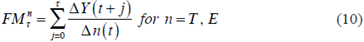
The transition variable is the output gap (Gy) and the cutting value is zero, that is to say, the two regimes are identified as growth and recession. The Fiscal Multiplier coefficient for a period τ is calculated as the accumulated response of Tax Revenue or Expenditure to an exogenous shock to the government expenditure shock:9
In other words, the degree of FM measures the change in accumulate response in output up to moment τ in the presence of an exogenous or autonomous shock in the respective fiscal indicator in period 0. Appendix C describes, step-by-step, how we estimate FM coefficients under the Bayesian approach.
6. Results
6.1 Model comparison and selection
Table 2 shows the natural logarithms of Bayesian Factors (BF) for each of the models to a restricted zero-lag model (a model with only one constant term)10. It is assumed as independent (i.e., we assign the same prior weight to each of the candidate models). Hence, the table reports the best alternative combinations of VAR, EST-VAR or LST-VAR, lag and delay (denominators) when compared to the restricted model with just intercepts (numerator). Hence, the closer the estimated BF is to zero, the more preferable the unrestricted model will be. In other words, the more negative “Ln(BF)” is, the better the specification obtained. The results (last column) show strong support for the LST-VAR non-linear specification for the transition variable output gap.
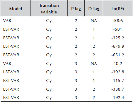
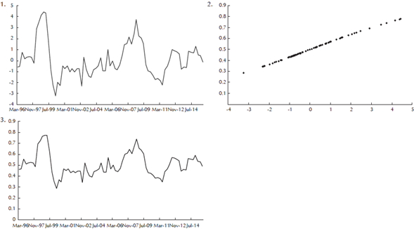
Therefore, the BF and the data seem to validate a logistic non-linear dynamics with two lags and a two-period delay for modeling the fiscal shocks on the GDP. In order to achieve a better comprehension of the non-linear effects, the dynamics of the transition variables and the estimated logistic transition functions, figure 2 shows graphical results of these estimations. On the top, the time series of the transition variable; at the center, their smooth transition functions, and at the bottom, the time profiles of the smooth transition function.
Accordingly, the non-linear impulse response functions and estimates of the FM coefficients reported below will be based on the results reported in Table 3.
6.2 Estimations of transition functions and their parameters
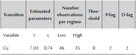
The estimation of the regression model given by equation (9) is done by the Gibbs sampler scheme described in Appendix C, which requires initial values. For the localization parameter c, the search is limited to the percentile range from 16%=cmin to 84%=cmax of the transition variable under consideration. As said before, the importance of parameter c is that it allows the regimes to be cataloged based on the values of the transition variable, for instance, positive or negative output gaps.
The results reported in Table 3 indicate that the estimated c is located fairly at the center of the distribution of the transition variable. For example, with our transition variable output gap, the 𝑐 estimate is 0.7, the threshold is 0.0, and the number of observations classified in the low regime is 46 and in the high, 35. In other words, the output gap has been in the negative regime in 57% of the cases along the sample.
In order to achieve a better understanding of the form of the non-linearity effects, the dynamics of the transition variable, and the estimated logistic transition functions, we plot the time series of the transition variable output gap (top), their smooth transition functions (center), and the time profile of the smooth transition functions (below) (Appendix A).
As the figure shows, the transition from one regime to another is smooth (central plot). Not only the trajectory of the variable (top), but also its historical transition function (lower), shows three critical moments throughout the sample. The first one may be related to the Colombian financial crisis in 1999, in which the output fell more than 4.0%. The second one could be due to the international financial crisis around 2009, which had a significant impact worldwide. The third one, at the end of the sample, has been caused mainly by the fall in international oil prices.
In summary, the transition functions seem to corroborate that the logistic smooth transition model and the transition variable output gap we selected are most likely to capture the non-linear behavior of FM embedded in the data.
6.3 Estimations of the degree and dynamics of FM
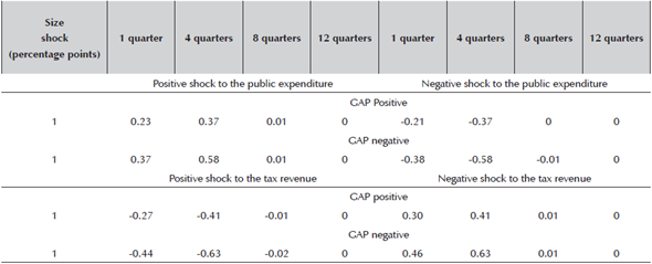
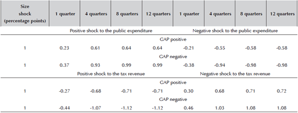
Tables 4 and 5 display values and dynamics of FM coefficients for different periods of time. Thus, the tables show the median of the impact and accumulated FM estimates (in percentage points) at each stage, conditional on each of the identified regimes of the output gap, in the presence of exogenous positive and negative 1.0% shocks in public expenditure and tax revenue. Notice that we took the median of FM rather than the mean because it is a more robust (resistant) measure to extreme values and it is preferred in cases where parameter distribution is asymmetric, as is the current case.
Table 4: Median Estimates of impact FM on GDP growth (Percentage points)
Source: Author's Calculations
Table 5: Median Estimates of Cumulated FM on GDP Growth (Percentage points)
Source: Author's calculations
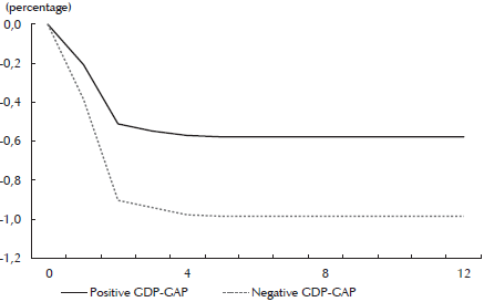
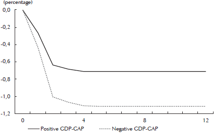
In addition, Figures 3, 4, 5 and 6 in Appendix B show the median of the time path of the cumulated FM coefficients when there is a positive and negative 1.0% shock to government expenditure and tax revenue for both regimes. From those figures, the reader can notice the non-linear nature of FM estimates for the state of the economy. The figures for other shock sizes are available upon request.
The minimum and maximum impact of the historical and accumulated Fiscal Multiplier at any time period τ can be summarized from tables 4 and 5. In the case of the impact FM, with a state of positive GDP gap and fiscal shocks that positively affect GDP (tax reduction or increase in spending), the highest FM is around 37% and 41% in the first year. While in a state of negative GDP gap, the FM reaches between 58% and 63% in the first year. The results are similar to shocks that negatively affect GDP (tax increase or reduction in spending).
Regarding the accumulated FM, with a state of positive GDP gap and fiscal shocks that positively affect GDP, the FM is between 24% and 26% in the first quarter and 62% and 68% in the third year. In the same state of the economy, but with shocks that impact the GDP negatively, the fiscal multiplier reaches between -23% and -28% in the first quarter and -60% and -70% in the twelfth quarter. On the other hand, under a state of the economy with a negative GDP gap, it is observed that the FM is around 38% and 45% in the first quarter and 97% and 109% in the third year with shocks that positively affect GDP. Finally, in the case of shocks that negatively affect GDP, the FM is around -38% and -45% in the first quarter and -97% and -110% in the twelfth quarter .
Thus, the evidence indicates the non-linear nature of the impact and accumulated FM. That is to say that the hypothesis that fiscal multipliers are dependent on the GDP gap is confirmed, showing that the economic cycle affects the form and persistence of fiscal multipliers, as was proposed by the IMF (2011). Particularly, it is found that the fiscal multiplier is higher in times of recession than in expansion, and that according to Batini, Eyraud, and Weber (2014), it is when production is below potential that it may have more persistent effects because of hysteresis effects (Delong & Summers, 2012; IMF, 2011), or because credit constrained agents cannot offset the reduction in their disposable income through borrowing. In comparison with Restrepo and Rincón (2006), our FM results are higher. However, the methodology that we use is different and our study period is broader. Therefore, it is not quite comparable.
Finally, the FM seems to respond slightly to the sign of expenditure and tax revenue. In other words, the FM appears to be symmetric in sign, since the degree of asymmetry is quite low if one compares the sizes of FM estimates.
7. Conclusion and final remarks
This article analyzes the non-linear effects of the tax revenue and expenditure multipliers for the Colombian case in the period between 1995-Q1 and 2015-Q4 through an LST-VAR model estimated using Bayesian statistical methods. The main findings were that the multipliers change depending on the state of the economy and does not depend on the sign of the shock. Therefore, their behavior is non-linear and symmetric. This had not been explored in the existing literature, and it is consistent with IMF (2010), when it was claimed that the business cycle also affects the persistence and shape of fiscal multipliers. In addition, tax revenue and expenditure multipliers appear to be slightly higher at times when the economy is in a recessive state and when the economy grows below potential output growth (negative output gap) than when it is in an expansive state. This is consistent with the Keynesian models, which state that the increase of public expenditure or the reduction of taxes can motivate the use of idle resources and increase the output when the output level of the economy is less than its potential caused by insufficient aggregate demand. This positive effect creates the possibility that the fiscal multiplier exceeds the unit since it increases in public expenditure or decreases in taxes. This induces increases in other components of expenditure demand (Sánchez and Galindo, 2013).
These results are consistent for several advanced countries, according to some studies that use a similar methodology, but frequentist in type (Blanchard & Leigh, 2013; Zangari, 2007; Mittnik & Semmler, 2010, Fazzari et al., 2011).
Another important finding is that tax revenue multipliers appear to be slightly higher than expenditure regardless of the state of the economy. This may be related to the fact that, in Colombia, expenditure is focused on areas that would not generate much impact on aggregate demand, whereas the tax policy would generate a great effect on agents’ decisions, such as the firms. According to many studies, Colombian companies make their decisions of production and investment depending on the regulation and tax stability. For example, Melo-Becerra et al. (2017) find that in the case of Colombia the effective tax rates are a key determinant in the investment decisions of companies in Colombia.
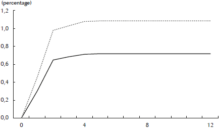
Another interesting fact is that, in general, all the multipliers are stabilized after the fourth quarter. This means that from then on, the impact that occurred in the zero period in tax revenue or expenditure stabilizes and the marginal effect is almost null. This also shows that fiscal policy is transmitted relatively quickly and stabilized after a short time, consistent with articles such as Ilzetzki et al. (2013).
Comparing the results, the tax revenue multiplier is above 1 in a state of the economy with a negative output gap. This result shows that an increase of one Colombian peso in the expenditure, the product is going to increase more than proportionally. This means that the tax policy could generate better results as an instrument of public policy and that it would also contribute more to stabilize the product in the short term.
Finally, our results have important policy implications, insofar as they enable the fiscal and monetary authorities of Colombia to better understand and monitor the impacts of the most important fiscal variables (taxes and expenses) on the aggregate demand depending on the state or regime in which the economy is in at that moment, in order to carry out its decision-making. The results obtained in this document, particularly the fact that the tax multipliers are higher, could contribute to better spending and tax policies (for example, tax reforms), as long as they are used as best policy instruments in the short term to impact the business cycle.