2.1 Conceptual Framework

Fiscal policy has a stabilizing effect on the economy if the budget balance-to-GDP ratio increases when output growth increases and falls when output growth declines: (i) the more countercyclical government spending is, the higher the effect of fiscal stabilization-a relatively high level of government spending when private demand is low will stabilize aggregate demand; (ii) the more pro-cyclical taxes are, the higher fiscal counter-cyclicality will be-if taxes fall more than output, when output falls, then taxes contribute to stabilize household’s disposable income.³

Assessing the degree of fiscal counter-cyclicality in each country i implies estimating the response of the budget balance to changes in economic activity:

where b is the budget balance-to-GDP ratio, Δy is a measure of changes in economic activity-proxied by GDP growth-and β measures the degree of fiscal counter-cyclicality, with larger values of the coefficient denoting higher counter-cyclicality.⁴

We then generalize equation (1) by introducing the assumption that the regression coefficients may vary over time:

In particular, the coefficients α and β is assumed to change slowly and unsystematically over time its conditional expected value to be equal to its past value. The change of the coefficient β is denoted by which is assumed to be normally distributed with expectation zero and variance ⁵

Equation (2) and (3) are jointly estimated using the Varying-Coefficient model proposed by ^{Schlicht (1985}, 1988). In this approach the variances are calculated by a method-of-moments estimator that coincides with the maximum-likelihood estimator for large samples (see Schlicht, 1985; Schlicht, 2003; Schlicht and Ludsteck, 2006 for more details).⁶ The model described in equation (2) and (3) generalizes equation (1), which is obtained as a special case when the variance of the disturbances in the coefficients approaches to zero.

As discussed by ^{Aghion and Marinescu (2008)}, this method has several advantages compared to other methods to compute time-varying coefficients such as rolling windows and Gaussian methods. First, it allows using all observations in the sample to estimate the degree of fiscal counter-cyclicality in each year-which by construction is not possible in the rolling windows approach. Second, changes in the degree of fiscal counter-cyclicality in a given year come from innovations in the same year, rather than from shocks occurring in neighboring years. Third, it reflects the fact that changes in policy are slows and depends on the immediate past. Fourth, it reduces reverse causality problems when fiscal counter-cyclicality is used as explanatory variable as the degree of fiscal counter-cyclicality depends on the past.

2.2 Fiscal counter-cyclicality over time

We now report the average level and the time path of the coefficient of fiscal counter-cyclicality estimated in equation (2) and (3) for a sample of 61 advanced and emerging market economies, for which we have estimates of fiscal counter-cyclicalityfor at least 20 years (Figure 1).

Source: Authors’ calculations.

Figure 1 Fiscal counter-cyclicality over time 

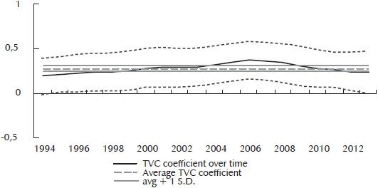
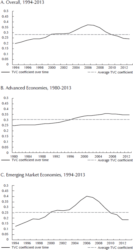
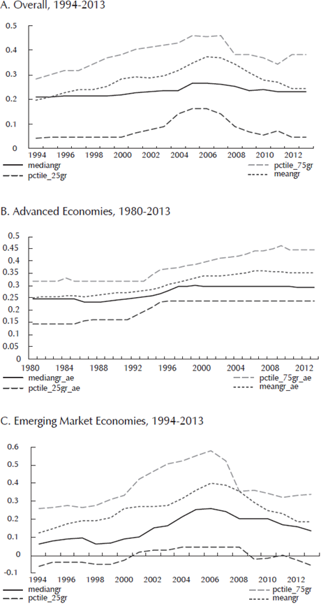
As a first observation, it is worth nothing that the time-average fiscal counter-cyclicality coefficient is positive (about 0.25-0.3), which is consistent with the fact that the budget balance is generally counter-cyclical ^{(Lane 2003}; ^{Aghion and Marinescu 2008)}. Second, the degree of fiscal counter-cyclicality has increased over time (Figure 1), for both advanced and emerging market economies (Figure 2), with the pattern holding for most countries within each group (Figure 3). In particular, the degree of fiscal counter-cyclicality has increased for 41 out of 61 countries in the sample.

Note: Figure displays the time profile of the TVC coefficient estimates for the entire sample, and two income groups, Advanced and Emerging Market Economies. A) includes 18 countries with at least 34 observations; B) contains 61 countries with at least 20 observations; C) contains 25 countries with at least 20 observations; D) contains 36 countries with at least 20 observations. Source: Authors’ calculations.

Figure 2 Fiscal counter-cyclicality over time 

Note: Figure displays the time profile of the TVC coefficient estimates for the entire sample, and two income groups, Advanced and Emerging Market Economies. A) includes 18 countries with at least 34 observations; B) contains 61 countries with at least 20 observations; C) contains 25 countries with at least 20 observations; D) contains 36 countries with at least 20 observations. Source: Authors’ calculations.

Figure 3 Fiscal counter-cyclicality over time, within sample 

However, while the increase in advanced economies has occurred mostly during the 80s and the 90s, in emerging market economies fiscal counter-cyclicality has increased in the late 90s-early 2000s. Interestingly, fiscal counter-cyclicality seems also to increase during recessions, particular during financial crises (Figure 4).

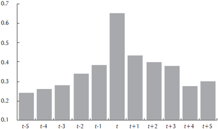
Note: Figure displays the average value of the TVC coefficient estimates from 5 years prior to the beginning of a given financial crises (“t”) to five years after it began. In each of the three panels averages were computed over a balanced sample. Source: Authors’ calculations

Figure 4 Fiscal counter-cyclicality during financial crises 

3.1 Empirical Methodology

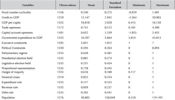
This section tests the importance of various macroeconomic and political factors in affecting the degree of fiscal stabilization. For this purpose, the following regression is estimated on a balanced sample of 61 countries for which we have estimates of fiscal counter-cyclicality for at least 20 years:

Where δi are country-fixed effects to capture unobserved heterogeneity across countries, and time-unvarying factors such as geographical variables which may affect the degree of fiscal counter-cyclicality ^{(Afonso et al. 2010)}; γ _t are time-fixed effects to control for global shocks; and X _it is a vector of time-varying macroeconomic and political variables ⁷

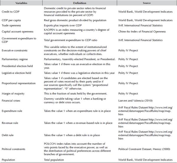
Macroeconomic variables:

Political variables:

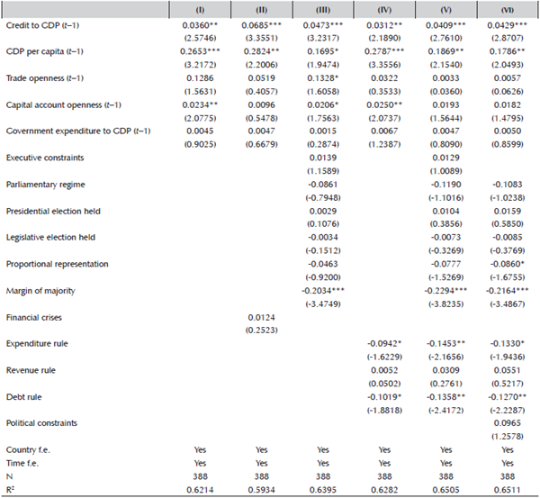
Since the dependent variable in equation (4) is based on estimates, the regression residuals can be thought of as having two components. The first component is sampling error (the difference between the true value of the dependent variable and its estimated value). The second component is the random shock that would have been obtained even if the dependent variable was observed directly as opposed to estimated. This would lead to an increase in the standard deviation of the estimates, which would lower the t-statistics. This means that any correction to the presence of this un-measurable error term will increase the significance of our estimates. To address this issue, equation is estimated using Weighted Least Squares (WLS). Specifically, the WLS estimator assumes that the errors in equation (1) are distributed as 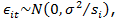where sit are the estimated standard deviations of the fiscal counter-cyclicality coefficient for each country i, and is an unknown parameter that is estimated in the second-stage regression. Finally, in order to reduce reverse causality, all the macroeconomic variables enter the specification with one lag.⁸

3.2 Results

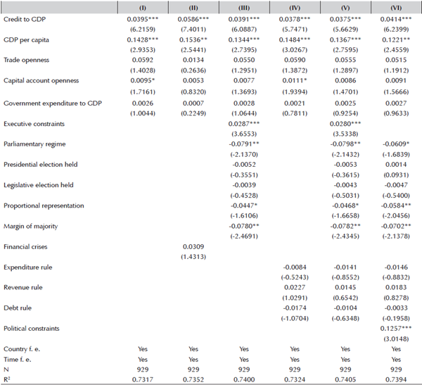
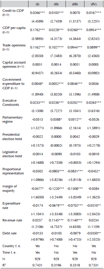
Table 1 presents the results obtained by estimating equation (4) using different econometric specifications. The coefficients associated with the various determinants typically exhibit the expected sign and confirm the conjectures discussed above.

Table 1 The determinants of fiscal counter-cyclicality 

Note: Results obtained by estimating equation (4). t-statistics in parentheses based on clustered robust standard errors. ***, **, * denote significance at 1,5,10 percent level, respectively.

Source: Authors’ calculations.

Starting with the set of macroeconomic variables, we find that fiscal counter-cyclicality is robustly and positively associated with the level of financial development, with an increase of 10 percentage points in the credit-to-GDP ratio increasing the degree of fiscal counter-cyclicality by about 0.2-0.3 (i.e. by about – -1 standard deviation). We also find that more developed and open to trade economies tend to have a larger degree of fiscal counter-cyclicality. Similarly, countries with larger government are also able to provide more stabilization, even though the magnitude is not economically significant: an increase of 10 percentage points in the government expenditure-to-GDP ratio increases fiscal counter-cyclicality only by about 0.05. Finally, we find that fiscal counter-cyclicality does not increase during financial crises once other macroeconomic variables are controlled for.⁹

Looking at the political variables, we find that constraints on the executive (constraint and polconv) are robustly and significantly associated with fiscal countercyclicality. The results are consistent with the evidence provided in ^{Fatas and Mihov (2013)} and ^{Lane (2003)}, who find that more constraints on the executive tend to reduce government spending volatility and positively influence overall fiscal stabilization. In contrast, all the other political variables, as well as dummies for fiscal rules, are not statistically significant.

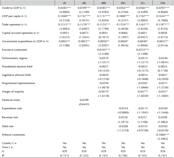
At the same time, some of these covariates tend to have different effects across country groups (Table 2 and 3). For example, while trade and capital account openness are negatively correlated with fiscal counter-cyclicality in advanced economies (as found by Aghion and Marinescu 20008), they are positively associated with fiscal counter-cyclicality in emerging market economies. Similarly, government size tends to have larger effect in advanced than in merging market economies, while the opposite is true for financial development.

Table 2 The determinants of fiscal stabilization - Advanced Economies 

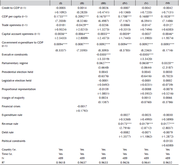
Note: Results obtained by estimating equation (4). t-statistics in parentheses based on clustered robust standard errors. ***, **, * denote significance at 1,5,10 percent level, respectively.

Source: Authors’ calculations.

Table 3 The determinants of fiscal stabilization - Non-Advanced Economies 

Note: Results obtained by estimating equation (4). t-statistics in parentheses based on clustered robust standard errors. ***, **, * denote significance at 1,5,10 percent level, respectively.

Source: Authors’ calculations.

As a robustness check, we replicated the results for the full specification by alternatively excluding country and/or time fixed effects. The results reported in Table 4 confirm the statistical significance of the macroeconomic variables. In addition, while constraints on the executive remain statistically significant across all specifications, we also find that some of the political variables that were not significant before in the baseline regression now become significant when country- and/or time-fixed effects are omitted. In particular, both proportional representation and expenditure rules turn out to be negatively and statistically significantly associated with fiscal counter-cyclicality across the various specifications II-IV.

Table 4 Determinants of Fiscal counter-cyclicality, alternative specifications 

Note: Results obtained by estimating equation (4). t-statistics in parentheses based on clustered robust standard errors. ***, **, * denote significance at 1,5,10 percent level, respectively.

Source: Authors’ calculations.

4.1 Empirical Methodology

This section examines the effect of fiscal counter-cyclicalityon output voliatility. For this purpose, the following regression is estimated based on a balanced sample of 61 countries for which we have estimates of fiscal counter-cyclicalityfor at least 20 years:

Where is the measure of fiscal counter-cyclicality estimated in the previous section for country i at time t; are country-fixed effects to capture unobserved heterogeneity across countries, and time-unvarying factors such a geographical variables which may affect the degree of fiscal counter-cyclicality and output volatility; are time-fixed effects to control for global shocks.¹⁰ denotes output volatility-measured by the absolute value of output gap- in country i at time t. The reason we use as baseline the absolute deviation of output gap is that this measures is available at yearly frequency and therefore allows to maximize the number of observations in our sample. To check the robustness of the results, we look at alternative measures typically used in the literature such as the standard deviation of the output gap or GDP growth. However, a problem with these measures in specification at yearly frequency is that they yield errors that are serially correlated within countries. We mitigate this concern when we consider 5-year non-overlapping panels.

In order to reduce endogeneity due to omitted variables that may simultaneously affect output volatility and fiscal stabilization, we include in the specification a set of control variables that have been found in the literature and in the previous section to be relevant: (i) trade openness; (ii) capital account openness; (iii) credit-to-GDP ratio; (iv) GDP per capita; (v) GDP growth; (vi) population; and (vii) government size. Moreover, all the macroeconomic variables enter the specification with one lag to minimize reverse causality. Equation (5) is estimated by Ordinary Least Squares (OLS) with robust clustered standard errors.

4.2 Results

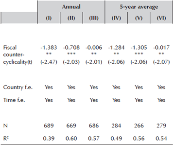
We start with a parsimonious specification of equation (5), using only country- and time-fixed effects as control variables. The results reported in Column I of Table 5 suggest that fiscal counter-cyclicality reduces output volatility. In particular, results suggest that an increase of 0.5 in our measure of fiscal counter-cyclicality (about 2 standard deviations) reduces output volatility by about ½ percentage point. In order to limit reverse causality, we reestimate this specification using the lag of fiscal countercyclicality. The results reported in Column II of Table 5 are similar and not statistically significantly different. Results are robust when the controls variables discussed above are included in the specification (Columns III-VI of Table 5), with that the effect of fiscal counter-cyclicality actually increasing, even though differences with respect to baseline estimates are not statistically significant. Among the control variables, we find that credit-to-GDP is positively associated with output volatility; while larger countries tend to be characterized by lower output volatility (this result is consistent with ^{Furceri and Karras 2007}). Interestingly, some of the variables such as trade openness, GDP per capita and government size-which are typically found to be associated with output volatility in cross-countries studies (for example, ^{Fatas and Mihov 2001}; ^{Debrun and Kapoor 2011})-are not statistically significant in our case. The reason for this relates with the inclusion of country-fixed effects which purge most of their variability. Indeed, they turn out to be significant when equation (5) is re-estimated by excluding country fixed effects (Columns II-III of Table 6).

Table 5 The effect of fiscal counter-cyclicality on output volatility 

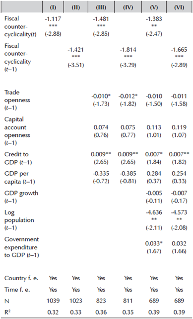
Note: Output volatility measured as the absolute value of the output gap. Results obtained by estimating equation (5). t-statistics in parentheses based on clustered robust standard errors. ***, **, * denote significance at 1,5,10 percent level, respectively.

Source: Authors’ calculations.

Table 6 The effect of fiscal counter-cyclicality on output volatility, alternative specifications 

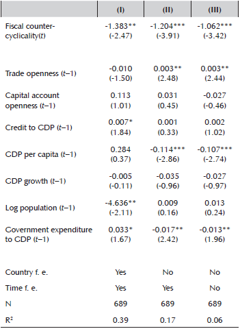
Note: Output volatility measured as the absolute value of the output gap. Results obtained by estimating equation (5). t-statistics in parentheses based on clustered robust standard errors. ***, **, * denote significance at 1,5,10 percent level, respectively.

Source: Authors’ calculations.

To account for the possibility that the relation between fiscal counter-cyclicality and output volatility has changed over time, we extend equation (5) by interacting the measure of fiscal counter-cyclicality with dummies for pre- and post-2000s, respectively:

The results obtained estimating equation (6) indeed suggests that the effect of fiscal counter-cyclicality on output volatility has increased over time (Column I, Table 5). Moreover, looking at the effect in the pre- and post-2000s periods and between advanced and emerging market economies, it seems that most of the increasing effect of fiscal counter-cyclicality on output volatility stems from the increase in fiscal counter-cyclicality in emerging market economies in the 2000s (Column II, Table 7). These results are consistent with the increase in the fiscal counter-cyclicality coefficient observed in many countries, particularly in emerging markets since the 2000s (Figure 1).¹¹

Table 7 The effect of fiscal counter-cyclicality on output volatility, across time and country samples 

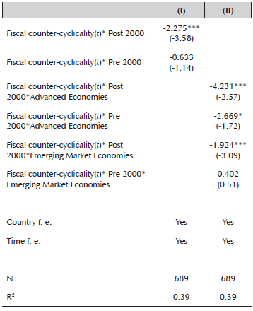
Note: Measure I= absolute value of the output gap; Measure II= standard deviation of the output gap on a five-year window; Measure III= standard deviation of GDP growth on a five-year window. Results obtained by estimating equation (6). t-statistics in paren theses based on clustered robust standard errors. ***, **, * denote significance at 1,5,10 percent level, respectively.

Source: Authors’ calculations.

Robustness checks

To check the robustness of our results we re-estimated equation (5) using alternative measures of output volatility: (i) the standard deviation of the output gap computed over a five-year rolling window; (ii) the standard deviation of GDP growth computed on a five-year rolling window.¹² The results presented in Columns I-III of Table 5, confirm that the fiscal counter-cyclicality reduces output volatility. In addition, the results are also robust when we estimate equation (5) on a five-year panel dataset using standard deviations computed on non-overlapping five-year windows.

Given that out measure of fiscal counter-cyclicality is based on estimates, we further check the robustness of our results by estimating equation (5) with WLS, giving more weights to observations for which the degree of fiscal counter-cyclicality is estimated more precisely. This procedure yields a larger effect of fiscal counter-cyclicality on output volatility (Column II, Table 8). In particular, an increase of 0.5 (about 1 standard deviation) reduces output volatility by about 1 percentage point.

Table 8.The effect of fiscal counter-cyclicality on output volatility,alternative measures and data frequency 

Note: Measure I= absolute value of the output gap; Measure II= standard deviation of the output gap on a five-year window; Measure III= standard deviation of GDP growth on a five-year window. Results obtained by estimating equation (5). t-statistics in parentheses based on clustered robust standard errors. ***, **, * denote significance at 1,5,10 percent level, respectively.

Source: Authors’ calculations.

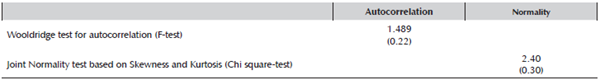
A concern estimating equation (5) using OLS is that the results may be subject to reverse causality since governments concerned with output volatility could arguably adjust their fiscal behaviors to provide more stabilization. While in principle this issue is likely to not be relevant in our case, as our measure of fiscal counter-cyclicality depends on the past, we check the robustness of our results using an IV approach. Following ^{Fatas and Mihov (2001}, 2013), we select instruments capturing institutional and political characteristics of the countries likely to be correlated to our measure of fiscal counter-cyclicality but presumably not directly related to output volatility. Based on the results presented in the previous section, we alternatively use the constraints on the executive variables (constraint and polconv) as instruments. Another instrument considered is the lags of fiscal stabilization. The results reported in Column III-IV of Table 9 confirms that fiscal counter-cyclicality reduces output volatility, with the effect being slightly higher (although not statistically different) than the one obtained with OLS. In addition, the Kleibergen-Paap test confirms the validity of the instruments.

Table 9 The effect of fiscal counter-cyclicality on output volatility, alternative estimators 

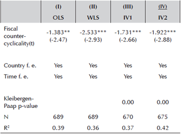
Note: Output volatility measured as the absolute value of the output gap. Results obtained by estimating equation (5). IV1= lagged fiscal counter-cyclicality and political constraints as instruments; IV2= lagged fiscal counter-cyclicality and polconv as instruments t-statistics in parentheses based on clustered robust standard errors. ***, **, * denote significance at 1,5,10 percent level, respectively.

Source: Authors’ calculations.