


 English (pdf)
 Article in xml format
 Article references
 Send this article by e-mail
 Cited by SciELO
  Cited by Google
  Similars in
SciELO
Similars in
SciELO  Similars in Google
 Permalink
1. Introduction
This paper assesses the technical efficiency of two key sectors for promoting economic development and social well-being: secondary education and health (Haini, 2020; Piabuo and Tieguhong, 2017). Given the economic and social pressures to reduce the fiscal deficit and prioritize public spending (for Latin America, see the ECLAC report, 2022), it is necessary to assess the efficiency of the sectors with the largest share of public budgets. This includes also considering the participation of the private sector in service provision, such as private schools and clinics.
For this purpose, a database with observations for developed and developing countries is used, although this requires a review process to exclude outlier observations, which is one of the main controls to be taken into account when working with the Data Envelopment Analysis (DEA) methodology. In particular, this study covers a total of 59 or 73 countries, depending on whether the secondary education or health sector is considered, and uses data from 2018.
It is worth mentioning that there are different methods to estimate the efficiency of a production process. Some are parametric since they are based on certain assumptions about the production functions and the probability distribution, this is the case of stochastic frontiers; others are considered non-parametric since they avoid this type of restrictions (e.g. FDH and DEA). In particular, we use DEA because it does not require assumptions about the production function since the estimates depend only on the observations we have, and it also allows us to consider the possible incidence of non-discretionary or environmental factors. However, Simar and Wilson (2007) show that the estimates in the second stage of the DEA, when it comes to studying the determinants of the level of inefficiency, present some complications, such as the lack of theory about the underlying process that generates the data and the assumption that the observations are independent of each other, so we prefer to use the bootstrap-based estimator that they propose.
This work is relevant because although many studies estimate technical efficiency across countries based on DEA, either for the secondary education sector (Afonso and Aubyn, 2006; Arias-Ciro and Torres-García, 2018; Aristovnik and Obadić, 2014) or for the health sector (Volkan and Serdal, 2006), they tend to focus on specific groupings, such as the OECD and the European Union. On the other hand, few developing countries are usually included in these studies, mainly due to lack of data.
Although other papers use monetary figures (e.g., expenditures) as inputs due to the difficulty of accessing physical units (Gavurova et al., 2017), this article avoids this practice due to the risk it entails, such as neglecting the incidence of different cost structures in the outcomes associated with the implementation of financial resources. Our work is also novel in the sense that there are relatively few publications on efficiency that include more than one sector (e.g., Afonso and Aubyn, 2005).
Indeed, the inclusion of more than one sector in the analysis allows us to determine whether technical efficiency in each sector depends more on institutional factors that may affect the processes of transformation of the resources that a country has to regulate and provide services, than on incidental aspects. In this regard, this work confirms the importance of GDP per capita and the level of corruption in explaining the level of sectoral efficiency, which also justifies the high correlation between the respective estimated efficiency indices. This suggests that there is some institutional learning, such that efficient countries in a particular sector can, at least in part, transfer their successful experience to other sectors.
In addition to this introduction, the paper consists of five other sections that can be considered stages in analyzing sectoral technical efficiency. First, some basic concepts are presented and some methodologies for estimating technical efficiency are described, so that the virtues of DEA are presented, taking into account the two-stage analysis and the model proposed by Simar and Wilson (2007). Then, the choice of the two sectors of interest for this study is justified, and the problems related to the choice of inputs and outputs are discussed. The third section describes the database and presents technical efficiency estimates. The fourth section discusses the results, and the fifth section includes the conclusions.
2. Conceptual and methodological framework
To measure the technical efficiency of a process, it is necessary to consider whether the factors of production (or inputs) are being used in the best possible way, without referring to what should be produced. To relate the quantities of inputs used to the products obtained, two alternatives can be proposed. In the first case, a productivity index could be used that relates the product (numerator) to the input (denominator); the other option is to compare the obtained result with the expected one, the latter estimated based on a set of explanatory factors.
If a productivity index is chosen, the answers to the questions of whether and to what extent a unit of analysis is efficient will depend on the cases included in the study, since the one for which a greater relationship is obtained will serve as a reference (benchmark) for others. What is said here assumes that the same production technology is available for all units of analysis, which suggests that they are relatively similar. On the other hand, when it comes to estimating a production possibilities frontier from a set of observations, this implies the need to choose a certain functional form, which is not free from criticism.
There are several methods for estimating the degree of technical efficiency, each with its pros and cons, but DEA and Stochastic Frontier Analysis stand out as being the most widely used. (Izquierdo et al., 2018; Mandl et al., 2008). On the one hand, DEA is based solely on the sample of decision-making units (DMU) and applies a linear optimization process considering the available observations, which avoids making assumptions about statistical distributions or production functions; at a cost, the results are sensitive to the inclusion of outliers or the composition of the sample (Mandl et al., 2008). On the other hand, stochastic frontier analysis allows us to test hypotheses statistically and assign them a certain level of confidence (i.e. it is a parametric approach), but assuming how inputs and outputs are related is difficult when traditional production processes are not involved.
For example, when conducting a technical efficiency analysis in sectors of public interest such as education, the first question is what to consider as inputs and what to consider as outputs. However, one would measure inputs by public and private expenditures allocated to the sector (which is questionable) and take some indicators of quality and coverage as outputs. In this case, the problem is to identify a process that convincingly links the two sets of variables.
In addition, the reader may wonder whether an increase in sector spending would be expected to lead to an increase in quality or coverage, or whether this would depend on other non-discretionary factors (e.g., the educational level of the parents or the socio-economic conditions of the student) and, most importantly, on how inputs are transformed into products.
Answering these questions is not trivial, even more so when a study extends to government interventions and their outcomes in areas such as equity and economic stability. The above is, of course, the result of assuming that many sectors of public interest (e.g., education, health, basic sanitation, or security) function as technical processes of transforming raw materials. In short, adopting any functional form to analyze efficiency in areas subject to government intervention will always be subject to criticism.
However, DEA is a good alternative for estimating technical efficiency in a transformation process, as long as it is controlled for outliers because it avoids making unfounded assumptions about the functional forms through which inputs and outputs are related. This methodology is based on a productivity index as a comparison criterion between DMUs but allows for multiple inputs and outputs in the process.
When there are multiple inputs and outputs, an obvious way to construct a productivity index is to monetize both the numerator and the denominator so that monetary units of product (e.g., sales) are related to the cost of production. Often, however, prices are not available, or it is not convenient to use them because of the different cost structures that may apply to each DMU. In this case, prices can be replaced by weights.
In general, the DEA considers that each DMU j is trying to solve a fractional problem (maximize
max
s.a.
To solve the previous (i.e., primal) problem, its dual modeling is usually considered because of the computational advantages this implies, especially when the number of DMUs is large relative to the total number of inputs and outputs. In addition, a convexity condition is often included to work with variable returns to scale (Charnes et al., 1978).
However, in addition to the inputs that can be modified by each DMU, its results may also depend on non-discretionary factors. For example, two countries with the same number of hospital beds and medical personnel might have different outcomes in the health sector because one of them might have more adverse environmental conditions (e.g., more pollution). In this regard, a traditional way to account for this fact has been to take the estimates of efficiency as the dependent variable in a censored linear regression model (i.e., a Tobit model with a limit at 1), which corresponds to a semi-parametric approach, so that these non-discretionary variables are introduced on the right side of the equation; this is known as two-stage DEA (Arias-Ciro and Torres-García, 2018). The above is shown in Equation 5, where δ j Ʌ represents the efficiency estimators while z jk is each of the non-discretionary factors.
Although this approach is commonly used in technical efficiency studies, Simar and Wilson (2007) have criticized it for two reasons: the lack of a theory of the underlying process that generates the data and the assumption that observations are independent of each other, which is difficult to justify given that sample selection affects efficiency estimation in DEA (i.e., the efficiency of a DMU depends on the combination of inputs and outputs of those units that are on the production frontier). The above can lead to serial correlation problems, which require caution when performing statistical inference.
Simar and Wilson (2007) have proposed a two-stage bootstrap-based estimator to generate the underlying data and statistically support estimates including non-discretionary factors. This model also allows for the adjustment of first-stage efficiency estimates (i.e., those obtained with the DEA), taking into account that certain characteristics of a DMU make it easier (or more difficult) to achieve efficient use of its inputs. Two countries with a similar allocation of inputs could achieve different levels of output, for example in areas such as education, depending on the socio-economic environment of the students, since if this is unfavorable (e.g., high dispersion of the population and poverty), it will also be necessary to articulate complementary policies that take into account these differences.
Consequently, the estimates of technical efficiency presented below are based on the Simar and Wilson (2007) model. This recognizes both the advantages of DEA (e.g., not being bound by predetermined functional forms) and its weaknesses (e.g., lack of knowledge about the underlying data generation process). In any case, a more detailed review of technical efficiency estimation methods and their advantages and disadvantages can be found in compilations such as Álvarez (2013) and Sickles and Zelenyuk (2019).
3. Secondary education and health: selecting inputs and outputs
The state can intervene directly or indirectly in various sectors that, by their characteristics, are a priority, either because of the negative effects that their deregulation would entail or, on the contrary, because they are essential to the fulfillment of the state’s mission. In particular, the literature tends to agree that it is not possible to achieve sustainable economic growth over time, improve the quality of life of citizens, or redistribute income if the state does not invest in education and health (Haini, 2020; Piabuo and Tieguhong, 2017). Moreover, this work focuses on these sectors to the extent that it is easier to identify potential inputs and outputs in them, at least compared to what would be expected if other areas of public interest were considered, such as distributive justice, macroeconomic stability, economic performance, institutional quality, and poverty (Afonso et al., 2005).
Regarding the education sector, we chose one of its levels, secondary education. This choice is due to the availability of data on aspects such as quality, given the existence of international tests carried out in several countries, such as those of the Program for International Student Assessment (PISA), as well as data on the resources used (e.g., teachers). The limitations of access to data at other levels of education are important so that at best there are observations for only a few countries, which must be taken into account here given the impact of the sample on the results of the DEA.
In the health sector, it is relatively easy to find statistics on mortality rates or life expectancy at birth, which correspond to the pair of variables traditionally taken as outputs in the literature (see, for example, Carrillo and Jorge, 2017; Volkan and Serdal, 2016). However, the number of observations changes depending on the set of inputs used. Although referring to public and private expenditures or to total expenditures, either as a percentage of GDP or per inhabitant, allows us to increase the number of DMUs in the analysis, which is also the case for the education sector, the problem with this is that it introduces biases due to the differences between the costs assumed by each study unit (i.e., country).
Indeed, the average salary of health care workers, for example, as well as the prices of other inputs (e.g., hospital beds), usually differ from country to country as a result of regulations (in the case of regulated salaries) and the game of supply and demand. Consequently, with the same budget (in a common monetary unit), different quantities of the same input can be purchased between countries, which makes it initially difficult to determine whether the efficiency indicators respond entirely to the input-output relationships achieved in the transformation processes or, at least in part, to the differences in the costs of the inputs used (Arias-Ciro and Torres-García, 2018). For this reason, we prefer to use physical quantities for the respective inputs in both sectors (secondary education and health), despite the loss of data that this implies, following the arguments of Afonso and Aubyn (2005).
For each of the sectors studied, two inputs and two products are used. For secondary education, the inputs and outputs are the number of teachers per hundred students, the number of computers per student, the average PISA test score, and the gross enrollment. Similarly, for the analysis carried out in the health sector, the variables used are the number of doctors, the number of hospital beds, the survival rate (per thousand inhabitants), and the life expectancy at birth. It should be noted that the choice of variables made here is based on the literature consulted (Afonso and Aubyn, 2005; Arias-Ciro and Torres-García, 2018; Carrillo and Jorge, 2017; Volkan and Serdal, 2016).
As mentioned above, the results that a country could achieve with a given allocation of inputs depend not only on how they are used but also on their context (Mandl et al., 2008). Therefore, it is necessary to consider other non-discretionary factors that could suggest adjustments to the efficiency indicators obtained in the traditional DEA analysis, leading to two-stage semi-parametric models (Álvarez, 2013; Arias-Ciro and Torres-García, 2018; Sickles and Zelenyuk, 2019). For the empirical exercise proposed here, the set of such variables includes GDP per capita and the corruption perception index provided by Transparency International.
The average level of income in a society is not only a proxy for the level of institutional development (Besley and Persson, 2013), but is also associated with, for example, the conditions under which students attend school or the health status of the population, through mechanisms such as nutritional intake and the degree of access to infrastructure (e.g., paved roads), drinking water and basic sanitation (Preston, 1976)1. For its part, corruption not only reduces the real quantity of inputs (e.g., cost overruns) but also indirectly affects their quality (Tanzi and Davoodi, 1997; Nguyen et al., 2017). Economic and political interests are more likely to prevail in matters such as the selection of teachers and medical staff when corruption is a common phenomenon2.
Although other factors could be considered, such as population size and density, because of their potential to capture the existence of economies of scale in the public and private provision of goods and services, they had to be excluded because they correlated with other non-discretionary factors (e.g., GDP per capita) and their low statistical significance in the second-stage regressions. Likewise, alcohol consumption per capita was initially included because it is associated with a higher likelihood of suffering from injuries due to accidents, poisoning, physical violence, and spontaneous abortions in the short term, while in the long term, it can cause, among other things, high blood pressure, heart defects, liver disease, and some types of cancer (e.g., in the mouth and throat) (Rehm et al., 2010; World Health Organization, 2019). However, this variable was not significant in the respective regressions, so it does not appear in the estimates.
4. Data and technical efficiency estimation
Table 1 presents the variables used in this paper, along with their description, the databases from which they were downloaded, and some basic statistics (mean, standard deviation, and minimum and maximum values). The data refer to the year 2018 for convenience (i.e., due to the availability of the figures). Only cases with observations for all variables to be used in the efficiency estimation, whether secondary education or health, were considered, so 64 and 78 countries, respectively, were initially included.
Table 1 Descriptive statistics of the variables used in the paper
| Inputs and outputs - Secondary education | |||||||
|---|---|---|---|---|---|---|---|
| Variable | Description | Source | Obs. | Mean | Stand. Desv. | Min. | Max. |
| Teachers | Number of teachers per 100 students | OECD | 64 | 3.785 | 0.728 | 2.276 | 5.303 |
| Computers | Number of computers per high school student | 0.662 | 0.356 | 0.078 | 1.608 | ||
| Educ_quality | Average score obtained by students from each country in the components of the PISA 2018 test, that is: mathematics, reading, and science | 458.055 | 49.248 | 334.119 | 556.470 | ||
| Enrollment | Percentage of students enrolled in secondary education compared to the population of age to attend the corresponding educational levels | World Bank | 107.422 | 18.020 | 63.117 | 155.961 | |
| Inputs and outputs - Health | |||||||
| Variable | Description | Source | Obs. | Mean | Stand. Desv. | Min. | Max. |
| Med_doctors | Number of medical doctors (and specialists) per thousand inhabitants | World Bank | 78 | 2.981 | 1.755 | 0.262 | 7.927 |
| Hosp_beds | Number of hospital beds per thousand people | 3.483 | 2.527 | 0.440 | 12.980 | ||
| Life_exp | The number of years a newborn is expected to live if current mortality rates do not change throughout his or her lifetime | 77.208 | 4.413 | 65.095 | 84.211 | ||
| Survival_rate | Number of children who survive the first year per thousand live births | 990.037 | 9.911 | 942.700 | 998.400 | ||
| Non-discretionary factors | |||||||
| Variable | Description | Source | Obs. | Mean | Stand. Desv. | Min. | Max. |
| GDP_per | Gross domestic product per capita based on purchasing power parity (in constant international dollars at 2017 prices) | World Bank | 64 | 36.485.230 | 21.320.010 | 7.446.936 | 115.049.900 |
| 78 | 31.784.220 | 22.092.490 | 4.369.762 | 115.049.900 | |||
| Corruption | Corruption Perception Index. The scale goes from 0 to 100, where 0 (100) is equivalent to the highest (lowest) level of perceived corruption | Transparency International | 64 | 57.516 | 18.298 | 28 | 88 |
| 78 | 52.987 | 19.653 | 16 | 88 | |||
Note: for the variables GDP_per and Corruption two mean values appear in each case since the number of observations depends on the sector being analyzed.
Source: Authors’ own elaboration based on data from the OECD, the World Bank, and Transparency International.
However, a disadvantage of DEA is its high sensitivity to outliers (Cylus et al., 2016), so it was necessary to review the data. Based on some box plots, it was observed that there were five countries with extreme values for their gross secondary enrollment rate (Jordan, with a value below 70%, and Belgium, Finland, Ireland, and Sweden, with values above 150%). Similarly, three countries (Burma, Pakistan, and Sudan) were found to have survival rates of less than 970 infants under one year of age per thousand live births, and two others (Japan and South Korea) had more than 12 hospital beds per thousand population. These atypical cases had to be excluded from the analysis, leaving 59 and 73 observations depending on the sector (i.e. secondary education or health).
Thus, the countries included in the estimation of technical efficiency in both sectors are Argentina, Austria, Brazil, Brunei Darussalam, Bulgaria, Canada, Chile, Colombia, Costa Rica, Czech Republic, Denmark, Dominican Republic, Estonia, France, Germany, Greece, Hungary, Iceland, Indonesia, Israel, Italy, Latvia, Lithuania, Luxembourg, Mexico, Montenegro, Morocco, the Netherlands, New Zealand, Norway, Peru, Poland, Portugal, Romania, Russia, Saudi Arabia, Slovakia, Slovenia, Switzerland, Turkey, the United Kingdom, the United States, and Uruguay.
The countries that appear in the estimates of technical efficiency only for the secondary education sector are Albania, Australia, Belarus, South Korea, Croatia, Georgia, Japan, Kazakhstan, Malaysia, Malta, Moldova, North Macedonia, the Philippines, Serbia, Singapore, and Thailand. On the other hand, the countries that are considered only for the health sector are the Bahamas, Barbados, Belgium, Bolivia, Sri Lanka, China, El Salvador, Spain, Finland, Grenada, Guatemala, Honduras, India, Iran, Iraq, Ireland, Jordan, Lebanon, Libya, Mongolia, Oman, Nicaragua, Qatar, Saint Lucia, Sweden, Suriname, Trinidad and Tobago, United Arab Emirates, Tunisia, and Egypt.
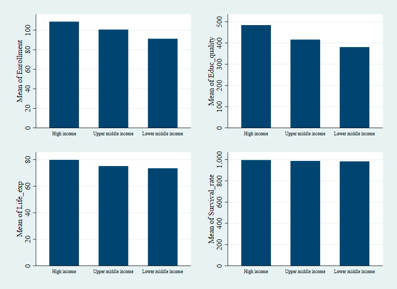
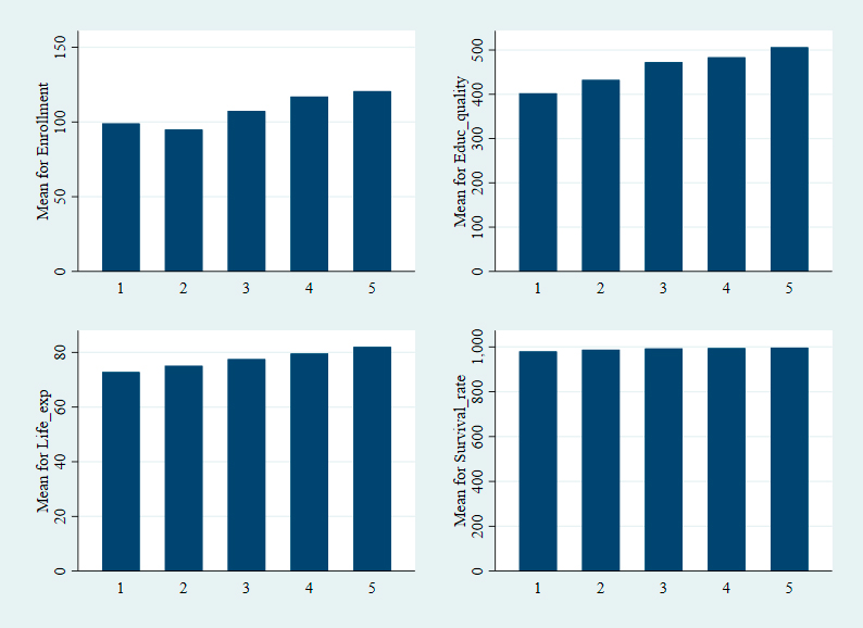
Before moving on to the estimates, the countries for which there are observations can be grouped according to their level of economic development, as classified by the World Bank (i.e., high, upper middle, lower middle, and low income)3. When the means of the four outputs considered in this document are then graphed by category (Graph 1), it is evident that the results are generally better for high-income countries, especially when the quality of secondary education is taken into account. This justifies the inclusion of GDP per capita as a non-discretionary factor in the two-step DEA.
Source: Authors’ own elaboration based on data from the OECD and the World Bank.
Graph 1 Average outputs by level of gross national income per capita
The previous exercise can also be done by grouping the means of the outputs according to the corruption perception index. However, the number of groups would be very large, so it was decided to look at the quintiles of the variable instead. Graph 2 shows something that was already raised when the inclusion of corruption as a non-discretionary factor was considered. Countries where this scourge is less prevalent also report better results in both areas.
Source: Authors’ own elaboration based on data from the OECD and the World Bank.
Graph 2 Average outputs by the perception of corruption
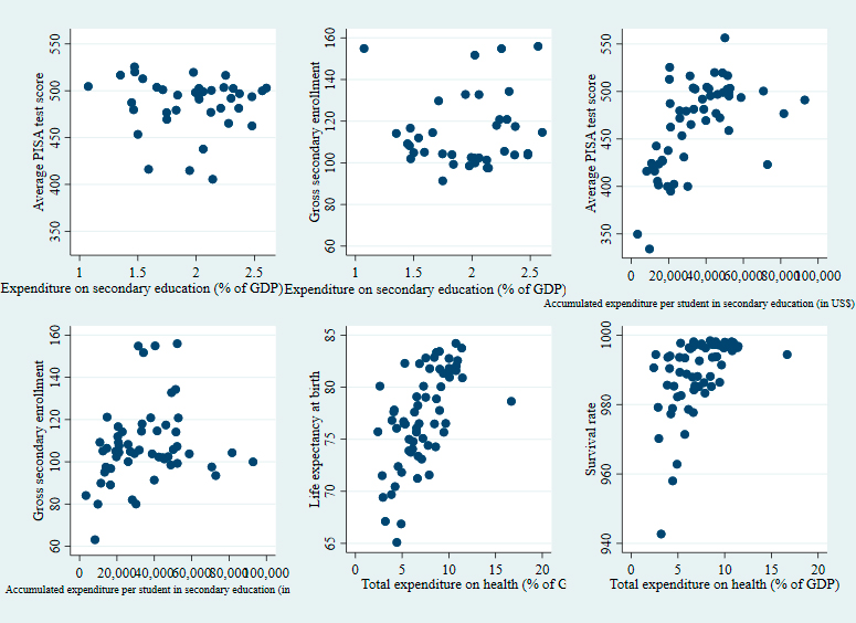
It is worth noting that the best results in education or health are not necessarily associated with higher spending in these areas, which also justifies the exclusion of inputs related to financing in the DEA analyses proposed later. Graph 3, which consists of a panel of scatter plots, shows that there is no association between total spending (public and private) on education (measured as a percentage of GDP) and both, average PISA test scores and gross enrollment in secondary education, which could be explained by differences in input costs across countries. However, when spending is measured as the total US dollars invested on average by each 15-year-old student in secondary education from the beginning of their education (early childhood), there seems to be a positive relationship with our quality proxy (i.e., PISA test score). Spending on health, on the other hand, seems to be positively associated with life expectancy at birth but not with survival rate.
Source: Authors’ own elaboration based on data from the OECD and the World Bank.
Graph 3 Scatter plots between outputs and sectoral spending levels
Now, to estimate the technical efficiency in each sector, we use, as already explained, the model proposed by Simar and Wilson (2007). This tries to solve some problems associated with estimating the determinants of efficiency in a second step after applying the DEA (e.g., correlation). Moreover, the estimates presented below are output-oriented, since it would be unreasonable to propose reductions in the quantities of inputs, taking into account social resistance and the need to make progress in aspects such as the quality of education or life expectancy at birth in many countries, especially in developing countries.
Table 2 shows estimated technical efficiency indices based on Shephard’s distance measure (inverse distance weighting) rather than Farell’s (radial). Therefore, the indices belong to the range [0, 1] rather than [1, ∞]; in both cases, the value 1 is assigned to the most efficient DMUs. This table shows the unadjusted and adjusted efficiency indices for the incidence of non-discretionary factors, in addition to the ranking of each country.
Table 2 Technical efficiency in secondary education and health sectors
| Education | ||||
|---|---|---|---|---|
| Country | Efficiency (DEA) | Adjusted efficiency | DEA ranking | Adjusted ranking |
| Poland | 1 | 0.975 | 1 | 1 |
| Estonia | 0.986 | 0.973 | 6 | 2 |
| Denmark | 0.987 | 0.957 | 5 | 3 |
| Australia | 0.992 | 0.955 | 4 | 4 |
| Slovenia | 0.974 | 0.955 | 7 | 5 |
| South Korea | 1 | 0.953 | 1 | 6 |
| Netherlands | 1 | 0.951 | 1 | 7 |
| Singapore | 1 | 0.951 | 1 | 8 |
| United Kingdom | 0.967 | 0.949 | 10 | 9 |
| Canada | 0.968 | 0.946 | 9 | 10 |
| Japan | 1 | 0.945 | 1 | 11 |
| Portugal | 1 | 0.942 | 1 | 12 |
| Greece | 0.992 | 0.939 | 3 | 13 |
| New Zealand | 0.951 | 0.937 | 11 | 14 |
| Norway | 0.951 | 0.933 | 12 | 15 |
| Thailand | 1 | 0.93 | 1 | 16 |
| Germany | 0.948 | 0.926 | 13 | 17 |
| Swiss | 0.935 | 0.919 | 17 | 18 |
| Saudi Arabia | 0.973 | 0.919 | 8 | 19 |
| Costa Rica | 1 | 0.917 | 1 | 20 |
| Iceland | 0.931 | 0.917 | 18 | 21 |
| Uruguay | 1 | 0.917 | 1 | 22 |
| Russia | 0.928 | 0.911 | 19 | 23 |
| France | 0.935 | 0.91 | 16 | 24 |
| Mexico | 0.994 | 0.909 | 2 | 25 |
| Latvia | 0.921 | 0.906 | 25 | 26 |
| Italy | 0.925 | 0.905 | 21 | 27 |
| Hungary | 0.925 | 0.902 | 22 | 28 |
| Israel | 0.942 | 0.902 | 15 | 29 |
| Czech Republic | 0.919 | 0.901 | 27 | 30 |
| Belarus | 0.918 | 0.898 | 28 | 31 |
| Croatia | 0.924 | 0.894 | 23 | 32 |
| Lithuania | 0.905 | 0.889 | 31 | 33 |
| Montenegro | 0.944 | 0.887 | 14 | 34 |
| Türkiye | 1 | 0.885 | 1 | 35 |
| Malt | 0.904 | 0.882 | 32 | 36 |
| Austria | 0.899 | 0.882 | 34 | 37 |
| USA | 0.903 | 0.882 | 33 | 38 |
| Luxembourg | 0.891 | 0.881 | 35 | 39 |
| Serbia | 0.922 | 0.877 | 24 | 40 |
| Chile | 0.908 | 0.874 | 30 | 41 |
| Argentina | 0.927 | 0.868 | 20 | 42 |
| Albania | 0.919 | 0.865 | 26 | 43 |
| Kazakhstan | 0.908 | 0.865 | 29 | 44 |
| Moldova | 0.887 | 0.848 | 36 | 45 |
| Brazil | 1 | 0.839 | 1 | 46 |
| Slovakia | 0.859 | 0.838 | 39 | 47 |
| Colombia | 0.883 | 0.833 | 37 | 48 |
| Malaysia | 0.87 | 0.823 | 38 | 49 |
| Philippines | 1 | 0.822 | 1 | 50 |
| Morocco | 1 | 0.822 | 1 | 51 |
| Bulgaria | 0.828 | 0.81 | 42 | 52 |
| Brunei Darussalam | 0.823 | 0.807 | 44 | 53 |
| Peru | 0.848 | 0.805 | 40 | 54 |
| Romania | 0.824 | 0.804 | 43 | 55 |
| Georgia | 0.841 | 0.797 | 41 | 56 |
| Indonesia | 0.817 | 0.767 | 45 | 57 |
| North Macedonia | 0.779 | 0.747 | 46 | 58 |
| Dominican Republic | 0.711 | 0.677 | 47 | 59 |
| Health | ||||
| Country | Efficiency (DEA) | Adjusted efficiency | DEA ranking | Adjusted ranking |
| Estonia | 1 | 0.999 | 3 | 1 |
| Finland | 1 | 0.999 | 5 | 2 |
| Ireland | 1 | 0.999 | 2 | 3 |
| Slovenia | 1 | 0.999 | 1 | 4 |
| Norway | 1 | 0.999 | 6 | 5 |
| Luxembourg | 1 | 0.999 | 1 | 6 |
| Montenegro | 1 | 0.999 | 1 | 7 |
| Iceland | 1 | 0.999 | 1 | 8 |
| Czech Republic | 0.999 | 0.999 | 9 | 9 |
| Italy | 1 | 0.999 | 4 | 10 |
| United Arab Emirates | 0.999 | 0.999 | 8 | 11 |
| Poland | 0.999 | 0.999 | 7 | 12 |
| Qatar | 1 | 0.999 | 1 | 13 |
| Swiss | 1 | 0.998 | 1 | 14 |
| Austria | 0.999 | 0.998 | 10 | 15 |
| Portugal | 0.999 | 0.998 | 11 | 16 |
| Canada | 1 | 0.998 | 1 | 17 |
| Sweden | 1 | 0.998 | 1 | 18 |
| Lithuania | 0.998 | 0.998 | 21 | 19 |
| Germany | 0.998 | 0.998 | 18 | 20 |
| New Zealand | 0.999 | 0.998 | 15 | 21 |
| Denmark | 0.999 | 0.998 | 14 | 22 |
| Belgium | 0.999 | 0.998 | 16 | 23 |
| Hungary | 0.998 | 0.998 | 20 | 24 |
| Israel | 0.999 | 0.998 | 12 | 25 |
| Latvia | 0.998 | 0.998 | 22 | 26 |
| Netherlands | 0.998 | 0.998 | 17 | 27 |
| Spain | 1 | 0.998 | 1 | 28 |
| Lebanon | 0.999 | 0.998 | 13 | 29 |
| France | 0.998 | 0.998 | 23 | 30 |
| United Kingdom | 0.998 | 0.998 | 24 | 31 |
| Greece | 0.998 | 0.998 | 26 | 32 |
| USA | 0.998 | 0.997 | 25 | 33 |
| Saudi Arabia | 0.998 | 0.997 | 28 | 34 |
| Slovakia | 0.997 | 0.996 | 30 | 35 |
| China | 0.998 | 0.996 | 27 | 36 |
| Russia | 0.996 | 0.996 | 33 | 37 |
| Costa Rica | 1 | 0.996 | 1 | 38 |
| Oman | 0.997 | 0.996 | 29 | 39 |
| Brunei Darussalam | 0.997 | 0.996 | 32 | 40 |
| Bulgaria | 0.996 | 0.995 | 38 | 41 |
| Romania | 0.996 | 0.995 | 37 | 42 |
| Chile | 0.996 | 0.995 | 35 | 43 |
| Türkiye | 0.996 | 0.995 | 34 | 44 |
| Uruguay | 0.996 | 0.995 | 39 | 45 |
| Sri Lanka | 1 | 0.995 | 1 | 46 |
| Iran | 0.996 | 0.994 | 36 | 47 |
| Peru | 1 | 0.994 | 1 | 48 |
| St. Lucia | 0.998 | 0.994 | 19 | 49 |
| Mexico | 0.997 | 0.994 | 31 | 50 |
| Libya | 0.994 | 0.994 | 41 | 51 |
| Bahamas | 0.994 | 0.993 | 43 | 52 |
| El Salvador | 0.994 | 0.993 | 42 | 53 |
| Argentina | 0.993 | 0.993 | 46 | 54 |
| Morocco | 1 | 0.992 | 1 | 55 |
| Brazil | 0.992 | 0.991 | 50 | 56 |
| Jordan | 0.992 | 0.991 | 49 | 57 |
| Colombia | 0.992 | 0.991 | 51 | 58 |
| Tunisia | 0.994 | 0.991 | 44 | 59 |
| Nicaragua | 0.996 | 0.991 | 40 | 60 |
| Barbados | 0.991 | 0.99 | 53 | 61 |
| Egypt | 0.993 | 0.99 | 45 | 62 |
| Guatemala | 1 | 0.989 | 1 | 63 |
| Grenade | 0.991 | 0.989 | 52 | 64 |
| Surinam | 0.992 | 0.989 | 48 | 65 |
| Mongolia | 0.987 | 0.987 | 57 | 66 |
| Honduras | 1 | 0.987 | 1 | 67 |
| Indonesia | 0.993 | 0.986 | 47 | 68 |
| Trinidad and Tobago | 0.986 | 0.985 | 58 | 69 |
| Bolivia | 0.988 | 0.985 | 56 | 70 |
| Iraq | 0.989 | 0.985 | 54 | 71 |
| India | 0.988 | 0.98 | 55 | 72 |
| Dominican Republic | 0.98 | 0.978 | 59 | 73 |
Source: Authors’ own elaboration.
Table 3 shows the estimates of the second stage, in which the efficiency index is correlated with the non-discretionary variables, namely GDP per capita and the perception of the level of corruption. The natural logarithms of these factors are included in the respective models to interpret the coefficients as semi-elasticities.
5. Analysis of the results
When the averages of the efficiency indices adjusted for the incidence of non-discretionary factors are compared by sector, it is found that the respective figure for secondary education is lower than for the health sector; in the first case it is 0.887 and in the second it is 0.995. This indicates that there would be more room to increase outputs in secondary education using the same resources, by 11%, in contrast to what happens for health, in which outputs could increase on average only 0.5%. Part of the justification for this result is found in the respective quantities of outputs since the relative dispersion is lower for the variables Life_exp and Survival_rate compared to Educ_quality and Enrollment. From Table 1 it can be seen that the relative standard deviations of these variables are 5.72%, 1%, 10.75%, and 16.77% respectively.
Under input-oriented estimates, the margin for reducing the amount of inputs while maintaining product levels (i.e., under an input-oriented model) is greater. The averages of technical efficiency concerning inputs for the secondary education and health sectors are 0.777 and 0.700 respectively. This suggests that increasing outputs from relatively high levels is generally costly, so their increase is marginal even when inputs are used efficiently.
In comparative terms, the estimates of technical efficiency that we obtain here are below the levels usually found for secondary education or health sectors in other studies (e.g., Arias-Ciro and Torres-García, 2018; Carrillo and Jorge, 2017). Although this is a characteristic of analyses based on DEA, a situation that can favor this tendency is the composition of the sample since such studies usually include relatively similar countries or territorial entities of the same nation. For its part, the database used in this study is more heterogeneous, which also explains a greater dispersion in the efficiency indicators, especially concerning secondary education.
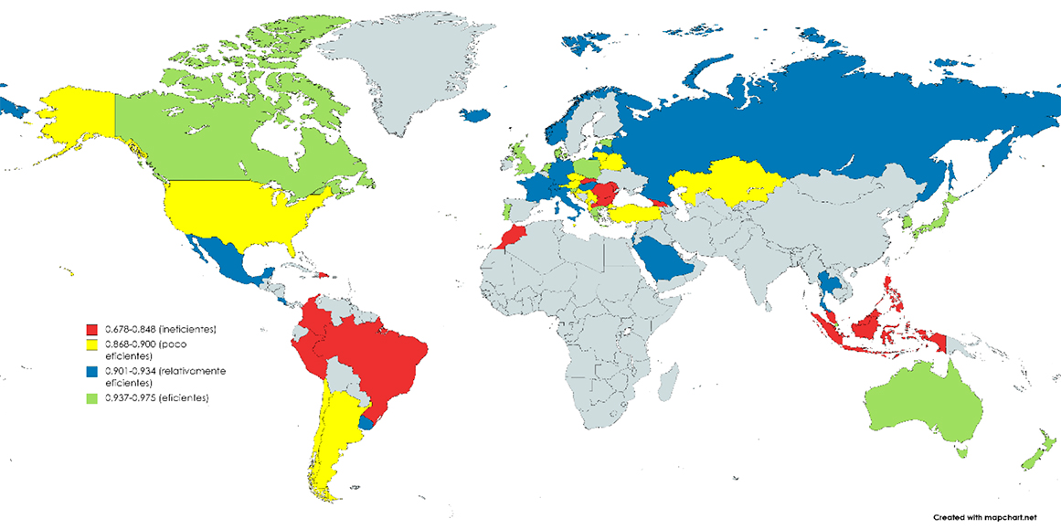
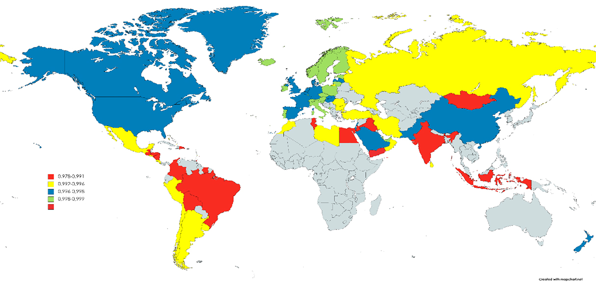
Another way to visualize efficiency in each sector is to identify the respective quartiles and then associate a color to each one, ranging, for example, from red (for the least efficient countries) to green (for the most efficient). Figures 1 and 2 refer to the maps obtained for secondary education and health. Although differences are observed between the two figures, it is noteworthy that no countries are identified that are very efficient in one sector and not very efficient in the other (i.e., if a country appears highlighted in green on a map, it will not be highlighted in red on the other).
This suggests that behind technical efficiency there are institutional factors that can favor or hinder the adequate management of the resources available, which is in line with the estimates of the second stage of the DEA (Table 3). However, it is not about replicating management models between sectors according to their results regarding technical efficiency, since what works in one scenario will not necessarily work in another. Thus, successful practices must be adjusted according to the particularities of each sector, a process whose speed will depend on the capacity of organizations (e.g., ministries) to validate and adjust their routines (Castañeda-Rodríguez, 2011).
The Pearson correlation coefficient between the adjusted efficiency indices for secondary education and health is 0.807, while the Spearman correlation is 0.605. However, these statistics consider only 43 countries, which are the common cases in both estimates.
It should be remembered that the level of economic development is usually taken as a proxy for the institutional capacity of a state (Besley and Persson, 2013). In this regard, the results indicate that a 1% increase in a country’s GDP per capita or a 1% increase in its corruption perception index is associated with a 0.043% and 0.086% increase in the level of technical efficiency in secondary education, respectively. Similarly, for the health sector, the corresponding elasticities are of the order of 0.008% and 0.003%, which is reasonable given that the efficiency indices in this sector are relatively high and not very dispersed (relative deviation of 0.479% from the average).
It is worth emphasizing that just as better results in education and health are not necessarily achieved with more resources, technical efficiency is not achieved by spending more. To demonstrate this, it is sufficient to calculate the correlation indices between these variables. In this respect, the correction between the adjusted efficiency index in the secondary education (health) sector and the sectoral expenditure as a percentage of GDP is -0.122 (0.402).
If we now focus on the six countries with the highest technical efficiency in secondary education, i.e. Poland, Estonia, Denmark, Australia, Slovenia, and South Korea (Table 2), we find that they also have better coverage indicators and quality compared to the average. The same is true in the health sector, where the most efficient countries also have above-average performance (in the case of Estonia, Finland, Ireland, Slovenia, Norway, and Luxembourg). Among the “top 6” of technical efficiency in the two sectors, Estonia and Slovenia stand out for appearing in both lists, which is consistent with what was mentioned about the high correlation between the efficiency indices.
Therefore, achieving high rates of technical efficiency in both sectors is associated with obtaining relatively large amounts of output, which helps explain some findings of other authors (e.g., Aristovnik and Obadic, 2014; Gavurova et al., 2017). For example, of the six countries with the lowest efficiency rates in secondary education (i.e., the Dominican Republic, North Macedonia, Indonesia, Georgia, Romania, and Peru), three (Dominican Republic, Indonesia, and Romania) employ a lower-than-average number of teachers and computers per student and also have low levels of gross enrollment and PISA test scores. It is not surprising, then, that the country with the lowest efficiency indices in education (i.e., the Dominican Republic) also has the worst performance figures, with a gross secondary enrollment rate of 79.9 percent and an average PISA test score of 334.12 points.
In the health sector, of the six countries with the lowest efficiency indices (i.e., Dominican Republic, India, Iraq, Bolivia, Trinidad and Tobago, and Indonesia), five (except Trinidad and Tobago) have a lower than the average number of doctors and hospital beds per thousand inhabitants. In turn, the six countries exhibit life expectancy at birth and survival rates below average. Furthermore, India, Iraq, and Bolivia are among the five nations with the lowest life expectancy at birth and survival rates in the sample.
The above can be corroborated through scatter graphs that relate both inputs and outputs to the adjusted efficiency indices. Graphs 4 and 5 indicate that there are no apparent associations between the quantities of inputs and levels of efficiency in secondary education and health. However, this changes when inputs are replaced by outputs so that countries that achieve better results in each sector tend to show high rates of technical efficiency.
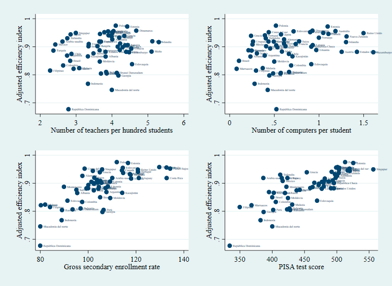
Source: Authors’ own elaboration.
Graph 4 Relationships between inputs, outputs, and efficiency in secondary education
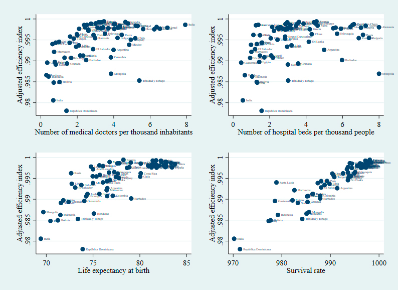
Source: Authors’ own elaboration.
Graph 5 Relationships between inputs, outputs, and efficiency in health
All of this suggests that we should consider the practices of those countries that have higher levels of coverage and quality in their secondary education systems, or that have higher life expectancy at birth and child survival rates. Therefore, we conclude this section by discussing some practices common to the countries that occupy the top positions in the efficiency rankings.
The countries that occupy the top five positions in the efficiency ranking for secondary education (i.e., Poland, Estonia, Denmark, Australia, and Slovenia) are characterized by two things. First, they are characterized by public funding that aims to provide free education at the primary and secondary levels and to reduce the impact of students’ context on their academic success. In addition, these countries focus on the quality of teachers and administrators so that the best students are encouraged to enter the teaching profession, and their updating is required with a certain frequency.
The five countries with the highest technical efficiency in healthcare, namely Estonia, Finland, Ireland, Slovenia, and Norway, also have predominant public sector involvement in the provision of services. In all of these countries, for example, primary health care is guaranteed by the state. It is usually free of charge for citizens who do not have the financial means to pay for it. At the same time, specialized medical services generally require additional payment or must be purchased from private providers, albeit with some cost controls. In Norway, in particular, the state is responsible for health care at all levels, but moderating quotas are set to rationalize demand.
These health systems additionally incorporate some criteria for the provision and qualification of medical personnel. In this sense, nurses usually treat some less complex illnesses (e.g., the flu) to avoid congesting medical care, in the same way that a family doctor is assigned to health users and is responsible for evaluating and referring to specialists. It is also common to use integrated information systems through which health-providing entities share patients’ medical histories, which avoids reprocessing and allows epidemiological controls to be carried out, for example. Regarding the practice of health professionals, continuous training and the presentation of periodic proficiency tests are required (e.g., in Ireland, they are annual and random).
6. Conclusions
This study first estimates technical efficiency in two sectors that are fundamental for any country, secondary education and health, not only because of their positive externalities but also because of their share in public spending. In such cases, it is necessary to determine whether the resources used are well utilized, or whether more outputs could be obtained with the same amounts of inputs, taking into account, for example, the circumstances under which the services are provided. In this regard, we find that output-oriented technical efficiency is on average lower in secondary education than in health, since it is 0.887 in the former and 0.995 in the latter, applying a two-stage DEA analysis to a sample of 59 and 73 countries, respectively.
However, an interesting point behind these results is that there are institutional factors that can contribute to a country’s better or worse comparative performance since the transformation of inputs into outputs is context-dependent. For example, the results show that an increase in GDP per capita (corruption perception index) by 1% is associated with a 0.043% (0.008%) and 0.086% (0.003%) increase in technical efficiency in secondary education and health, respectively. Moreover, countries that are efficient in one sector tend to be efficient in the other; the Pearson correlation index between the corresponding adjusted efficiency indices is 0.807. At this point, it is worth highlighting the cases of Estonia and Slovenia, which appear simultaneously in the “top 6” of technical efficiency in education and health (Table 2).
Similarly, the paper shows that the most efficient countries in each sector are those that produce greater quantities of outputs, not necessarily those that use fewer inputs. Furthermore, the achievement of above-average outputs is not generally associated with the monetary resources used (e.g., expenditure). The six countries with the highest technical efficiency in secondary education, i.e., Poland, Estonia, Denmark, Australia, Slovenia, and South Korea, have better coverage and quality indicators than the average. The same is true in the health sector, where the most efficient countries also show good results in terms of life expectancy at birth and child survival (e.g., Estonia, Finland, Ireland, Slovenia, Norway, and Luxembourg). The correlation between the adjusted efficiency index and the outputs is greater than 0.715 in all cases. This indicates the importance of deepening the study of the sectoral practices of the most technically efficient countries.

