Mario Linares Vásquez¹, Diego Fernando Hernández Losada² y Fabio González Osorio³

¹ Ingeniero de Sistemas, Universidad Nacional de Colombia. Candidato M.Sc., Ingeniería de Sistemas y Computación, Universidad Nacional de Colombia. Auxiliar docente, Departamento de Ingeniería de Sistemas e Industrial. mlinaresv@unal.edu.co
² Ingeniero Industrial. Magíster, en Administración de Empresas. Magíster en Economía. M.Sc., of Science in Finance. Ph.D., en Ciencias Económicas. Profesor, Departamento de Ingeniería de Sistemas e Industrial y Decano, Facultad de Ingeniería, Universidad Nacional de Colombia. dfhernandezl@unal.edu.co
³ Ingeniero de sistemas. Magíster, en Ciencias Matemáticas, Universidad Nacional de Colombia. M.Sc. in Computer Science, The University of Memphis, USA. Ph.D, in Computer Science, The University of Memphis, USA. Profesor asociado, Departamento de Ingeniería de Sistemas e Industrial y Decano, Facultad de Ingeniería, Universidad Nacional de Colombia. fagonzalezo@unal.edu.co

ABSTRACT

Selecting an investment portfolio has inspired several models aimed at optimising the set of securities which an investtor may select according to a number of specific decision criteria such as risk, expected return and planning horizon. The classical approach has been developed for supporting the two stages of portfolio selection and is supported by disciplines such as econometrics, technical analysis and corporative finance. However, with the emerging field of computational finance, new and interesting techniques have arisen in line with the need for the automatic processing of vast volumes of information. This paper surveys such new techniques which belong to the body of knowledge concerning computing and systems engineering, focusing on techniques particularly aimed at producing beliefs regarding investment portfolios.

Keywords: portfolio, optimisation, stock, securities, return, risk, profile, belief, rules set.

RESUMEN

El proceso de selección de portafolio ha dado origen a diferentes modelos, orientados a optimizar el conjunto de titulos valor disponibles para un inversionista, con base en diferentes criterios de decisión tales como el riesgo, el retorno esperado, horizonte de planeación, entre otros. El enfoque clásico de estos modelos cubre las dos fases del proceso de selección de portafolio, y está definido por disciplinas tales como la econometría, el análisis técnico y las finanzas corporativas. Pero el nacimiento de la computación financiera define el uso de nuevas técnicas bajo la necesidad del procesamiento automático de grandes volúmenes de información. Este artículo es un estado del arte de esas nuevas técnicas, desde el punto de vista de la ingeniería de sistemas y sus modelos computacionales, aplicados particularmente a la generación de expectativas de inversión en portafolios.

Palabras clave: portafolio, optimización, acciones, títulos valor, retorno, riesgo, expectativas, conjunto de reglas.

Recibido: octubre 01 de 2007
Aceptado: febrero 21 de 2008

The financial market has become one of the main components of capitalist economies; it is an elementary mechanism for raising capital, transferring risks and international trade. Investment is an activity which is tightly bound to financial markets. It basically consists of buying and selling (stocks, commodities and currency) aimed at making profit. It is a game where all internal and external variables involved in the process must be correctly interpreted for producing beliefs; such beliefs are decision-making variables in the decision-making process.

Portfolio selection represents a specialisation of investment in the stock market domain, framed within the conceptual framework of finance; it consists of selecting a set of securities available on the market, according to an investor’s profile and requirements. Decision-making is defined by an investtor’s ability to understand stocks’ historical behaviour and the influence of external factors such as micro and macro-economic environments. Intuition, knowledge and good luck are examples of components which are generally recognised as being factors in successful portfolio selection.

The classical framework for portfolio selection is defined by the risk/return element of Markowitz’s theory (Markowitz, 1952). This theory states that portfolio selection consists of two stages: creating beliefs and portfolio design; the former concerns how investors define their beliefs about markets’ future performance whilst the latter deals with how investors select investments according to their own beliefs. Several mathematical and probabilistic models have been developed from a financial viewpoint for the design stage; however, they have assumed that beliefs are represented as probabilistic distributions of stock series data. Econometrics provides models for time series analysis (re creating beliefs), including forecasting, regression and function approximators regarding stock series data; technical analysis (Murphy, 1999) provides charts and technical indicators suggesting beliefs about market trends to the investors. However, beliefs are not only density functions of stock data, nor values concerning market trends; beliefs in the real world are rules and patterns repre-senting the investor’s knowledge and ability to understand market dynamics. Classical financial models thus do not support this type of representation but several computer-based techniques can handle such representations (using rules, patterns, etc.) and are widely used in the academic community.

This survey is thus aimed at presenting several computational models found in the literature for solving the problem of creating portfolio beliefs. Initially of this survey presents a conceptual framework for selecting a portfolio as part of a multi-objective optimisation approach, presents classical models for portfolio design (being the second stage of the process), presents models for creating beliefs concerning portfolio performance, focusing on statistical and computational techniques. Finally draws conclusions and proposes further work on computational techniques for creating beliefs.

The portfolio selection problem

Portfolio selection is described as being the selection of a se-curities set from an available universe; such selection is driven by a decision-maker’s objectives and according to an investor’s knowledge and beliefs about market behaviour. The aim behind this selection is to invest a limited amount of money for a period of time on securities bringing an investor the best expected values concerning the variables involved in decision-making. The aim then (from the viewpoint of eco-nomics) is to maximise investor wealth. The following information categories are involved:

-Quantitative: indices, technical indicators, security prices (time series); and

-Qualitative: fundamental beliefs, news, speculation.

An investor acting within a classical and rational economics’ environment will thereby wish to invest in stocks producing the highest return; however, the decision concerning which stocks to choose (i.e. those forming the portfolio) is orientated by beliefs such as the price of stock “x” is going down because the dollar price is high.. or, I will not invest in stock “y” because its price has gone down since last week[...]. Such rules describe how knowledge about stock performance arises according to factors such as the market, the stocks’ history, political decisions, the economic environment and speculation. An investor’s profile is then defined by the following:

-Position: geographical position, job, sociological and economical conditions;

-Preferences: risk attitude, time conditions, expected return; and

-Predictions: trading rules, beliefs, stock trends and so on.

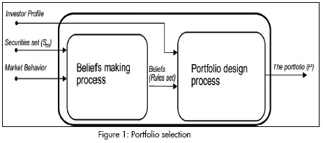
Two stages are involved in portfolio selection (Markowitz, 1952); the first consists of creating beliefs about securities’ performance in horizon planning (the time during which an investor is going to take portfolio decisions). An investor must observe market behaviour and use experience and knowledge of domain application in creating such beliefs. Output from this stage results in a set of rules subjectively describing securities’ performance (predicted behaviour). The set of rules or beliefs generally represent probability distributions for securities, association rules, temporal patterns, trading rules and so on.

The second stage consists of using beliefs about securities for designing a portfolio. This selection is defined by an investor’s objective variables. The set of securities and the vector of money invested in each selected security represent the output from this stage. This output is called a portfolio and is applied to an investment period; a sequence of portfolios must be built (one for each period) when an investor is working with multiple periods. This sequence is called a portfolio selection algorithm (El-Yaniv, 1998) and specifies how an investor must reinvest wealth from period to period (Figure 1).

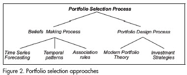
Several approaches have been found in the literature for providing a solution for the portfolio selection problem. However, these approaches do not cover the whole process; they have been developed for a specific stage of the process (Figure 2). The models are organised in document according to the stages and notation defined below.

Portfolio selection may be generally defined as being multiobjective optimisation. The investor’s profile directs the process and is defined by multiple objective variables and constraints such as the expected stock yield, the decision-maker’s risk profile, horizon planning and the amount of money available for the investment. Portfolio selection is formally defined in a multi-objective approach as follows:

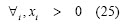
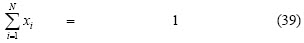
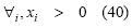
With Sm a set of available securities on the market, and a horizon planning H with L time periods, then the portfolio selection problem consists of finding a portfolio P of N securities for each period of H, with P ={ S_P, x^*} where S_P S is the portfolio securities set, and [x^* = x₁^*, x₂^*,...., x_n^{* T}] is the vector of wealth proportions invested in each security of S_P . The portfolio must satisfy the investor profile, so x^* will satisfy:

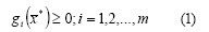
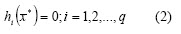
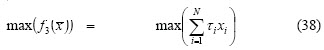
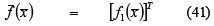
and optimise

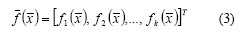
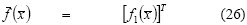
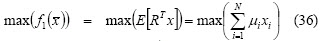
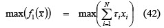
The investor profile is represented by equations (1), (2) and (3). So (1) and (2) define the feasible region and represent the constraints imposed on the process; the k components of (3) represent the main criteria for portfolio selection. For example, a classical investor would prefer f₁ = max(return) while an investor adopting a return-risk approach would prefer f₁ = max(return) and f₁ = min(risk).

Return and risk concepts

Return (yield) and risk represent the main concepts in portfolio selection, these being the main objective variables driving the whole process. Return is the profit or yield obtained as a result of investment; it is a security or portfolio’s gain or loss during a particular period, consisting of income plus capital gains relative to investment. Return is usually quoted as a percentage.

Risk is commonly defined as being the chance or possibility that a real investment return will be different from what was expected; it is also referred to as being the uncertainty involved in an investment in a security or portfolio. In economics, risk measures the expected loss for an investment in monetary units. Risk is defined by the factors influencing any securities’ performance. Risk is generally classified as follows:

-Systematic risk (pervasive risk), affecting a large number of securities. For example, the effect of political news on stock prices is a kind of systematic risk. Systematic risk is a product of the financial market’s dynamics. It is thus impossible to protect an investor against this or try to predict it; and

-Specific risk (unsystematic risk), influencing individual assets or a specific set. Such influence on portfolio selection can be reduced through diversification. This principle is based on the fact that specific risk influences tend to become cancelled out in large and well-diversified portfolios.

Both types of risk compound a security’s total risk, so a security risk consists of adding systematic risk to specific risk.

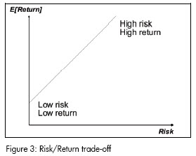
The implicit relationship between risk and return defines the conceptual framework for a decision-makers’ interaction with the market. This trade-off between return and risk is repressented by the decision-maker’s profile or risk tolerance (adverse to risk, risk-lover) and is expressed on the market by the fact that higher-risk investments have higher expected return. Expected return may involve a loss proportional to risk with higher-risk values (Figure 3). The investment game is thus played with risk/return trade-off investor management.

Measuring return

Portfolio selection includes evaluating stock series performance; these series are considered to be random variables. A decision-maker has thus to rely on a toolbox of measurements and indicators describing stock behaviour. Stock series are described in terms of portfolio selection by measuring central tendency and return dispersion. Risk is thus represented by returns’ variance and return on the expected value of the returns’ series. These measurements are used on the assumption than stock returns follow normal distribution.

The return is obtained from the stock series prices⁴ as a random variable transformation so return also becomes a random variable. This transformation is defined as a real function:

with Y(t) a time series of security prices and k is the regression time window. Simple return and log return are two instances of (4) which are widely used in finance.

Simple return

This is also called an arithmetic return and is defined with k=1 as follows:

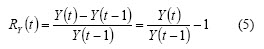
A simple return with k window size is called k-step:

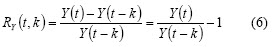
This return has some features:

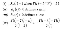
Log return

A simple return is an asymmetric function regarding positive and negative changes of the same magnitude. For example, if Y(t) = 13 and Y(t-1) = 8, then simple return R_Y (t) = 0.625, but if Y(t) = 8 and Y(t - 1) = 13, R_Y (t) = -0.3846. Log (logarithmic) return fixes simple return asymmetry and is defined as follows:

and with k-step:

This return has some features:

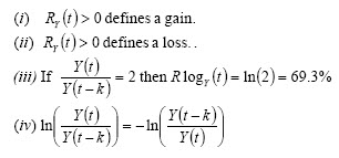
Risk measurement

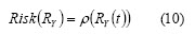
Multiple measurements allow an investor to estimate an investment’s financial risk (Giorgi, 2002; Galvan, 2004; Nawrocki). These kinds of measurements are functions g of the securities’ return (range Rⁿ and domain R):

Equation (9) represents the set of functions which can be considered as a risk measurement. Artzner et al., (1999), reduced the functions set g to ρ, with risk measurement axiomatisation and coherent risk measurement definition:s

with ρ a coherent risk measurement is defined as follows:

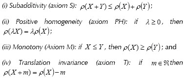
-Axiom S is related to the diversification theorem. If portfolio risk is not less than the sum of individual risks, then an investtor would prefer to invest in securities individually and not on a portfolio.

-Axiom PH. The risk of λ units of X is equal to λ times the risk of X; it is a consequence of axiom S.

-Axiom M. If return X is less than return Y, then risk ok X will be higher.

-Axiom T. Risk decreases if the portfolio has a risk-free security.

Coherent risk evaluates the risk associated with future states while classical risk measurement assesses risk with return historical data.

Convex risk measurement is an extension of coherent ones. Convex measurement is a weak form of coherent measurement. Convex measurement includes situations in which risk position⁵ does not increase lineally with position size:

A function ρ : X → R is called convex measurement if it fulfils the conditions of convexity⁶, mononotony and translation invariance.

Variance and semi-variance are classic risk measurements and belong to a group called deviation measurement:

A function ρ : X → R is called deviation measurement if it fulfils the following conditions (in addition to subadditivity and positive homogeneity):

A set of risk measurements widely used in portfolio selection are presented below.

Variance

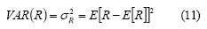
Risk is associated with the volatility of securities’ prices and securities returns in a classic conception. Assuming that returns’ data has symmetrical and normal distribution, then expected return represents central tendency and variance is average variation with mean:

Semi-variance

This is based on the observation that decision-makers do not worry about the risk of securities having prices below a threshold. Semi-variance is an answer for handling securities having asymmetric distributions and is defined as follows (Deng et al., 2000):

with being the time series data and the threshold. A particular instance of semi-variance occurs when the threshold is the expected value:

Semi-variance defines risk as being the volatility below the threshold and is a particular case of a set of measurements called K-th order lower partial moments (LPMk)⁷.

VaR: value at risk

VaR involves the concept of providing a simple number encapsulating all available risk portfolio information (Rom-bouts and Rengifo, 2004). This number must be understood by people lacking financial skills and the operations involved in calculating it must be fast. VaR is based on two aspects of the financial market:

-Managers measure risk as loss in monetary units; and

-Portfolio deviations less than expected return do not have the same probability as deviations exceeding expected return (i.e. distribution of returns is not symmetric concerning central tendency).

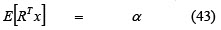
VaR thus measures the dispersion of loss associated with a fixed occurrence probability (α level). Higher risk means higher loss with a fixed probability. For a level α ∈ [0,1], VaR is defined as follows:

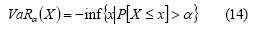
VaR is not a coherent risk measurement because it does not fulfil the subadditivity axiom.

ES: expected shortfall

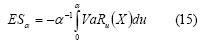
Expected shortfall is a solution for VaR weakness (i.e. expec-ted shortfall fulfils the subadditivity axiom). Expected shortfall with an α level is average loss in the worst 100 • α%:

Portfolio design

The following notation will be used in this section:

- x_i: proportion invested in security i

- R_i: return for i-th security; random variable with μ_i = E[R_i]

- R = [R₁,R₂,...,R_n]^T

- µ = [µ₁,µ₂,...,µ_n]^T

- COV(R): variance-covariance matrix of random vector R

- W(t): the investor’s wealth for period t

The purpose of this stage is to build optimal portfolio P. This is based on Markowitz’s Modern Portfolio Theory (MPT) (Markowitz, 1952 and 1999) which has inspired a lot of work on the nature of portfolio selection. Two approaches in the literature cover portfolio design: MPT and investment strategies (Van der Hart et al., 2001; Amir et al., 2002); this survey focuses on the former.

The purpose of the MPT approach is to build a portfolio according to return and risk decision criteria. Models arising from such dual decision criterion have been developed according to the measurement used for evaluating risk (i.e. risk interpretation is the main element of MPT models). Decision criteria in earlier models (before MPT) only consisted of maximising return but, with the introduction of the concept of portfolio diversification, risk became an important element in new models of portfolio selection.

Mean and variance models

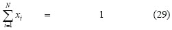
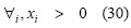
This kind of model assumes normal securities’ probability distribution and represents beliefs about securities’ future performance. Mean distribution is considered as return while variance is the measurement used for risk. Mean-variance models have assumed that an investor is averse to risk. The available wealth for an investor is 1, so . The model presents the following variations according to the constraints and objective functions which are used in the process:

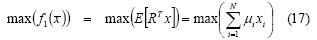
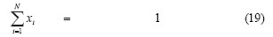
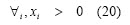
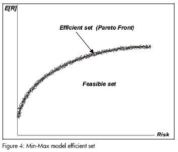
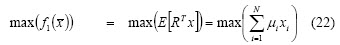
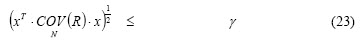
-Min-Max: This is the general case for the mean-variance model. Return maximisation and risk minimisation are the decision criteria applied in this mathematical model. The problem thus becomes multi-objective optimisation. The solution set is thus a Pareto front or efficient set (Figure 4 is an example of Pareto front for a Min-Max model). An investor must look at non-dominated solutions when selecting a portfolio and pick one of them according to his particular requirements. The model may be formally presented as follows:

-Max-return: The decision criterion was return maximisation with maximum value γ for risk:

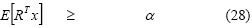
-Min risk: The decision criterion was variance minimisation with a minimum value α for return:

Portfolio diversification reduces securities’ specific risk but systematic risk is a market feature so it cannot be minimised with portfolios. Systematic risk affects securities’ return and establishes a relationship between market and security performance. This relationship is security β and is defined as follows:

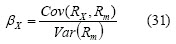
with R_x being the return for security X and R_m the market return.

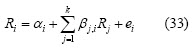
Sharpe proposed the CAPM model in 1963 (Sharpe, 1964), assuming that most stock prices increase when the market goes up and decrease when it goes down. A market factor is then introduced to describe such type of security movements. This market factor represents security β. Differences between individual securities’ returns are assumed to be the result of additional independent random disturbances specific to each security. A security’s return has two parts, the first depending on the market and the second being a random variable independent of other securities. The CAPM ex-pression is defined as follows:

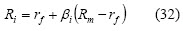
with r_f being the risk free rate on the market. Sharpe’s single index model states that a security’s return is a linear function of market return where the market is typically represented by one of the broad equity indices. Other factors different to market movement are observed to have an influence on security prices, such as the effects of industry and interest rates. Multi-index models have thus been proposed as a measurement involving several betas for systematic risk. The general form for multi-index models (with error e_i) is:

Mean-semi variance models (E-S)

Semi-variance measures risk in this model; it is proposed following the observation that investors may only be concerned with the risk of securities’ return being lower than the mean. It is not widely used in spite of its being intuitively closer to reality than the mean-variance model.

Mean absolute deviation model (MAD)

Mean-absolute deviation measures risk in this model (Kommo, 1991):

Skewness is the third momentum of a probability distribution measuring distribution asymmetry. This model is a natural extension of the mean-variance model which adds skewness as another criterion for portfolio selection (Deng et al., 2000) A third decision criterion is thus introduced: maximise expected skewness value. The MVS optimisation model has two forms:

-Max-Min-Max : if τ_i is the third momentum for the i-^th se-curity

-Max-skewness: if and are the target values for risk and return, respectively:

Creating beliefs making

Belief-making consists of producing a set of rules defining securities’ future performance. Many concepts, models and theories concerning which factors are involved in the securities’ temporal behaviour can be found in the literature (Chen et al., 1986; Burmesteir et al., 2003; Ekern, 1971). These factors or economic forces influencing all stock returns are known as systematic or pervasive risk and are the components making belief-making so interesting.

The beliefs are represented as rules. These rules are considerations about securities’ performance; the rules are also the knowledge hidden in the historical data. Three approaches for creating beliefs are presented below. Each has its own set of rules. Several computing and systems engineering techniques applied to belief-making are presented in this section. These techniques are classified into three groups:

-Time series forecasting;

-Association rules; and

-Interesting patterns and trends.

The first is the most widely used while the rest are attracting new followers within the computational finance community.

Time series forecasting

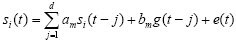
Securities forecasting is recognised in the community as being a very difficult task insofar as financial time series have special features (Hellstrom and Holmstrom, 1998; Rydberg, 2000). Two ways of modelling the problem from the point of view of data involved in prediction are commonly found in the literature: technical and fundamental analysis. Forecasting is only based on securities’ historical data in the former while fundamental analysis also includes data related to the market situation and other parameters. Technical analysis is based on the assumption that a particular stock’s historical performance is a strong indication of future performance. Formally, if s_i(t) is the predicted value for the i-^th security for time t, s_i(t) is defined for technical and fundamental analysis in (47) and (48), respectively, as follows:

In (48), I is a vector having the factors representing risk and other fundamental parameters which influence securities’ behaviour. The list below is an example of these factors:

-Inflation;

-Interest rates;

-Trade balance;

-Stock indices: Dow Jones, DAX, Swedish General Index; and

-Commodity prices: coffee, oil, currency.

Forecasting is formally defined as follows:

If S_i(t) is a time series for the i-^th security, w is the window’s autoregressive size, H is portfolio horizon planning and g(t) is a function of the factors involved in the process. Securities’ prediction thus consists of finding the values for s_i(t) in the following way:

In the case of technical analysis g(t)= 0.

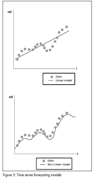
Prediction is formulated and solved according to two perspectives. The former assumes that the prediction model is linear; the second perspective is more general and defines the model as being non-linear. Figure 5 gives graphical examples of how data is represented by linear and non-linear models. The linear approach generally uses statistical techniques while the contemporary nonlinear approach is based on machine learning and evolutionary computation models. Predicting financial time series has therefore been solved in many ways, as follows:

-Linear autoregressive models (AR, ARMA, ARIMA Models), also called scoring models:

-Classical nonlinear models (Clements, 2003);

-Nonlinear models implemented with artificial neural networks;

-Evolutionary computation;

-Support vector machines; and

-Bayesian networks.

Neural networks

An artificial neural network is used as a universal approximator able to approximate any continuous function without a priori assumptions about the data. The aim of a neural network is to build an internal model (topology and connection values) for forecasting the desired values. The inputs are the s_i(t) available values and these are used for training and testing network sets. May strategies have been used for forecasting securities’ prices according to neural input and output:

-Input: individual prices, price combination, prices and technical indicator combinations; and

-Output: price forecasting, reversal point forecasting, index forecasting, candlestick forecasting⁸.

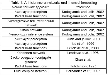
The literature presents models ranging from neural networks to time series forecasting (Kodogiannis y Lolis, 2002; Dunis y Jalilov, 2001; Lendasse et al., 2000; Lendasse et al., 1998; Chan et al.), such as recurrent neural networks, feed-forward networks with FIR filters and multilayer perceptrons; Hutchinson’s work (Hutchinson, 1999) using radial basis functions networks is a good example of this. Table 1 summarises the neural network approaches used in the literature for financial series forecasting.

Evolutionary computation

Evolutionary computation (EC) integrates evolutionary concepts with programming for solving hard optimisation problems. EC is implemented for stock forecasting via two approaches:

-Genetic algorithms (Koza, 1989).

-Genetic programming (Koza, 1992)

Genetic algorithms and genetic programming are used for finding non-linear models; in the genetic programming case, this process is called symbolic regression. For example, Kaboudan (Kaboudan, 2000) used symbolic regression with genetic programming for predicting stock prices.

Support vector machines (SVMs)

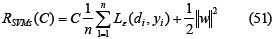
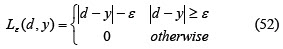
Applying SVMs to time series forecasting has become a subject of intense study from the perspective of non-linear regression stimation problems (Muller et al., Tay and Cao, 2001, Cao and Tay, 2001). SVMs estimate the regression function using linear functions which are defined in a high dimensional space. Given a set of G = {x_i,d_i}ⁿ (x_i is the input vector, d_i is the desired value and n is the space dimension) data points, the approximation function is:

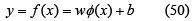
where Φ(x) is the high dimensional space and w and b are estimated by minimising

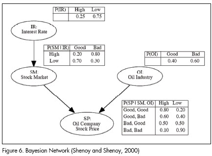
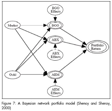
Bayesian networks (Heckerman, 1997)

A Bayesian network is a graphical model representing probabilistic relationships amongst variables of interest. Bayesian networks combine traditional quantitative analysis (historical data) with decision-maker judgment concerning qualitative information displayyed in a directed acyclic graph. The model’s output is a portfolio return distribution according to a Bayesian inference model (Shenoy and Shenoy, 2000). The network nodes represent the quantitative information while the edges represent the qualitative information. The nodes are thus the variables (stocks, indices) and the edges define variable dependencies (conditional probabilities between variables). Each variable has a set of mutually exclusive values called its state space (e.g. dollar price varies and its states are high or low). The model graphically represents the relationship between the factors affecting portfolio return, according to the network designer (Figures 6 and 7 are examples of Bayesian network portfolio models). The model depends on any combination of empirical data, investor expectations, judgment or forecast.

Association rules

An association rule defines a unidirectional relationship between two sets of attributes. It is an expression of the form if x then y which is supported by data, where x and y are predicates about problem attributes. So a predicate x is a logic expression with connectors . An example of an association rule in the financial field is something like if dollar increase = 0.1 and euro increase = 0.5, then x stock increase = 0.2. Association rules are also expressed as grammars and deterministic finite state automata when the rule has an associated output. Association rules state the interaction between securities, indexes series and market tendencies in portfolio selection.

The aim of data mining process is to automatically extract informative rules from the series. In most cases this means that the rules should have some level of precision, be repress-entative of the data, easy to interpret and interesting for a human expert (i.e. novel, surprising or useful). Association rules describe knowledge regarding an application domain. In the case of portfolio selection, the rules describes the knowledge implicit in the market behaviour or the beliefs which decision-makers (such as investors, experts and traders) have about market behaviour and securities’ performance.

Extracting rules can be applied to target securities and factors set S_T ⊆ S. A set of time series is analysed to find patterns or relationships between recurrent sets in the selected data. Data mining techniques, such as a priori algorithm and multidimensional association rules (Han and Kamber, 2001), are commonly used for rules extraction.

Shen has used an interesting rough sets (Pawlak, 1982) and SOM hybrid model for generating rules forming the input for a trading system. Rough sets is a mathematical tool for dealing with uncertainty (Shen and Loh, 2004). Rough sets have the following advantages in financial prediction:

-Integrated analysis of quantitative and qualitative attributes;

-Expressing knowledge in terms of natural language rules;

-Discovering knowledge in terms of data set key concepts; and

-Rough sets do not need any preliminary information about data, such as securities’ distribution probabilities or risk beliefs.

Shen used a rough SOM algorithm for transforming financial data into rough objects which are used to generate decision rules stating that if x then y, where x is a predicate of technical indicators and y is an investment strategy action.

Interesting patterns and trends

Discovering typical or frequents patterns is one of the current great challenges of mining databases containing time series data. An interesting pattern is a sequence of values which are common (or unusual) when collecting data, given a particular consideration. Temporal patterns occur frequently from the point of view of trends and seasonal effects in securities time series and in general financial series (Hellstrom and Holmstrom, 1998a and 1998b). The concept of seasonal effects states a relationship between series’ behaviour and calendar days; the calendar thus influences market and securities’ performance. The day-of-the week and month effect are e-xamples of how the academic community approaches financial series prediction.

Stock trends are also an interesting field in portfolio theory. This type of pattern has been widely studied, both theoretical and experimentally, for the followers of technical analysis.

Several models have been used for finding interesting patterns in securities’ series:

1. Prediction rules for data mining with genetic programming (Hetland and Saetrom, 2005);

2. Entropy and statistical dependency analysis (Darbellay and Wuertz, 2000; Cheng, 1999);

3. Temporal rules inference with SOM and recurrent neural networks (Giles et al., 1997); and

4. Clustering techniques.

The purpose of clustering is to group unsupervised objects into classes or clusters according to similarity measurement (Berkhin, 2002). Two rules govern the process:

-Minimise the distance between same cluster members; and

-Maximise the distance between clusters

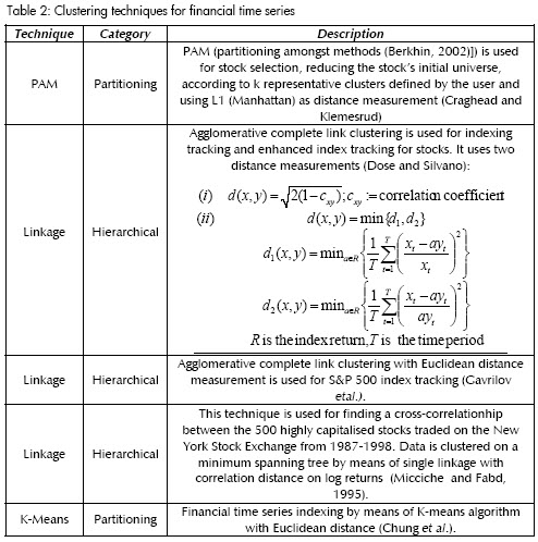
Clustering techniques are classified into hierarchical, partitioning relocation and density-based partitioning. Hierarchical clustering groups the data into a tree of clusters and is categorised into being agglomerative and/or divisive, according to the strategy used for building the tree (bottom-up, top-down). Partitioning clustering algorithms divide data into several sets in an iterative relocation process driven by greedy heuristics. Density-based methods group data according to concepts of density, connectivity and boundary. For more details about clustering techniques see Berkhin, 2002. Hierarchical and partitioning techniques have been used for universe reduction and stock indexing in portfolio selection in Craighead and Klemesrud, Dose and Silvano Cincoti, Gavrilov et al., Micciche and Fabd, 1995 and Chung et al. Table 2 summarises such techniques.

Conclusions and further work

The list of financial and computational models presented in this survey is a representative list of academic and scientific efforts aimed at solving the automatic portfolio selection problem. Each model presented here addresses one of the portfolio selection stages.

There is a financial and mathematical framework through which an investor can tackle the decision-making process in the case of optimal portfolio design. However, MPT models involve strong assumptions which (in most cases) are not appropriate for the several approaches which have been developed for creating beliefs. The survey presented several computational techniques applied to belief-making but also revealed how techniques such as fuzzy logic have not been explored. The reasoning involved in fuzzy logic may be considered as a strategy for modelling investor beliefs and may be mixed with data mining models for discovering market performance rules. Another interesting still to be explored area is the representation of time series as candlesticks; candlestick representation is a tool for technical analysis aimed at forecasting tendencies through visual chart analysis⁹. For example, Hernandez et al., (2007) used candlestick as a data representation scheme for stock forecasting with neural networks. This kind of representation may be useful for discovering interesting patterns using data mining and linguistic rules.

Further work in the field must be orientated towards integrating good practice and models for each stage in the process in a computer-assisted model helping an investor to build scenarios and portfolio efficient sets having the following features:

The model must involve quantitative and qualitative information in the belief building process;

Clustering and classification techniques must be used for extracting patterns and trends from historical data to support series forecasting and data mining for investment rules;

Correlation series analysis and data mining techniques must support knowledge extraction aimed at building portfolio design models and defining risk measurement;

Modern portfolio models must be applied to multi-period portfolio selection; and

Belief-building approaches (time series forecasting, extracting rules, pattern extraction, candlesticks) must support new portfolio design models.

4 A stock series has four prices: close, open, high and low.
5 A position represents an investment decision : buy, sell, hold.
6
7
8 Candlestick forecasting is the most recent approach. An example of this is given in (Hernandez et al., 2007) where multiple candlestick representations were used.

Bibliography

Amir, R., Evstigneev, I. V., Hens, T., ReinerSchenk-Hopp, K., Market selection and survival of investment strategies., Tech. Rep. 02-16, University of Copenhagen. Institute of Economics, Oct. 2002, available at http://ideas.repec.org/p/kud/kuiedp/0216.html.        [ Links ]

Artzner, P., Delbaen, F., Eber, J., Heath, D., Coherent measures of risk., Mathematical Finance, Vol. 9, 1999, pp. 203–228.        [ Links ]

Berkhin, P., Survey of clustering data mining techniques., technical report, Accrue Software, San Jose, CA, 2002.        [ Links ]

Burmesteir, E., Roll, R., Ross, S., Using macroeconomic factors to control portfolio risk., tech. rep., Insightful, 2003.        [ Links ]

Cao, L., Tay, F., Financial forecasting using support vector machines., Neural and Computing Applications, Vol. 10, 2001, pp. 184–192.        [ Links ]

Chan, M.-C., Wong, C.-C., Lam, C.-C., Financial time series forecasting by neural network using conjugate gradient learning algorithm and multiple linear regression weight initialization., Department of Computing, The Hong Kong Polytechnic University.        [ Links ]

Chen, N.-F., Roll, R., Ross, S. A., Economic forces and the stock market., Journal of Business, Vol. 59, No. 3, pp. 383–403, 1986. available at http://ideas.repec.org/a/ucp/jnlbus/v59y1986i3p383-403.html.        [ Links ]

Cheng, C.-H., Entropy-based subspace clustering for mining numerical data., Master’s thesis, Department of Computer Science & Engineering, Chinese University of Hong Kong, 1999.        [ Links ]

Chung, Fu,, T., Lai Ching, F., Luk, R., man Ng, C., Financial time series indexing based on low resolution clustering.        [ Links ]

Clements, M. P., Forecasting economic and financial time-series with non-linear models., Department of Economics University of Warwick, October 2003.        [ Links ]

Craighead, S., Klemesrud, B., Stock selection based on cluster and outlier analysis. Nationwide Financial.        [ Links ]

Darbellay, G. A., Wuertz, D., The entropy as a tool for analysing statistical dependences in financial time series., Physica A, D. Vol. 287, No. 3-4, 2000, pp. 429–439.        [ Links ]

Deng, X.-T., Wang, S.-Y., Xia, Y.-S., Criteria, models and strategies in portfolio selection,” AMO — Advanced Modeling and Optimisation., Vol. 2, No. 2, 2000, pp. 79– 103.        [ Links ]

Dose, C., Cincoti, S., Clustering of financial time series with application to index and enhanced-index tracking portfolio., tech. rep., Universit di Genova.        [ Links ]

Dunis, C., Jalilov, J., Neural network regression and alternative forecasting techniques for predicting financial variables., tech. rep., Liverpool Business School, 2001, pp. 15        [ Links ]

Ekern, S., Taxation, political risk and portfolio selection., Economica, Vol. 38, No. 152, 1971, pp. 421–30, available at http://ideas.repec.org/a/bla/econom/v38y1971i152p421-30.html.        [ Links ]

El-Yaniv, R., Competitive solutions for online financial problems., ACM Computing Surveys, Vol. 30, pp. 28–69, Mar. 1998.        [ Links ]

Gavrilov, M., Anguelov, D., Indyl, P., Motwani, R., Mining the stock market: Which measure is best?., tech. rep., Department of Computer Science- Stanford University.        [ Links ]

Giles, C. L., Lawrence, S., Tsoi, A. C., Rule inference for financial prediction using recurrent neural networks., in Proceedings of IEEE/IAFE Conference on Computational Intelligence for Financial Engineering (CIFEr), (Piscataway, NJ), IEEE, 1997, pp. 253–259.        [ Links ]

Giorgi, E. D., A note on portfolio selection under various risk measures., Tech. Rep. iewwp122, Institute for Empirical Research in Economics - IEW, 2002. available at http://ideas.repec.org/p/zur/iewwpx/122.html.        [ Links ]

Glavan, C. An application of alternative risk measures to trading portfolios., Master’s thesis, Finance School, Zurich University, 2004.        [ Links ]

Goldberg, D., Genetic algorithms in search, optimisation and machine learning., Addison-Wesley Professional, 1989.        [ Links ]

Han, J., Kamber, M., Data Mining: Concepts and Techniques., San Francisco: Morgan Kaufmann Publishers, 2001.        [ Links ]

Heckerman, D., Bayesian networks for data mining., Data Mining and Knowledge Discovery, Vol. 1, No. 1, 1997, pp. 79–119.        [ Links ]

Hellstrom, T., Holmstrom, K., Predicting the stock market., Tech. Rep. IMa-TOM-1997-07, Center of Mathematical Modelling - Malardalen University, August 1998a.        [ Links ]

Hellstrom, T., Holmstrom, K., Predictable patterns in stock returns., Tech. Rep. HEV-BIB-OP-30-SE, Center of Mathematical Modelling - Malarden University, 1998b.        [ Links ]

Hernandez, G., Linares, M., Rojas, S., On candlestick forecasting with an adaptive coupled dual neural network., in Memorias Congreso Internacional de Inteligencia Computacional CIIC 2007, 2007.        [ Links ]

Hetland, M. L., Saetrom, P., Evolutionary rule mining in time series databases., Machine Learning, Vol. 58, Feb 2005, pp. 107–125.        [ Links ]

Hutchinson, J. M., A radial basis function approach to financial time series analysis. Tech. Rep. AITR-1457, Massachusetts Institute of Technology, 1993.        [ Links ]

Kaboudan, M., Genetic programming prediction of stock prices,” Computational Economics., M. ol. 16, 2000, pp. 207– 136.        [ Links ]

Kodogiannis, V., Lolis, A., Forecasting financial time series using neural networks and fuzzy system-based techniques., Neural Computing and Applications, Vol. 11, 2002, pp. 90–102.        [ Links ]

Kommo, Y. H., Mean-absolute deviation model for portfolio optimisation and its application to Tokyo stock market., Management Science, Vol. 37, 1991, pp. 519–531.        [ Links ]

Koza, J., ed., Genetic Programming: On the Programming of Computers by Means of Natural Selectio., The MIT Press, 1992.        [ Links ]

Markowitz, H., Portfolio selection., Journal of Finance, Vol. 7, 1952, pp. 77–91.        [ Links ]

Lendasse, A., Bodt, E. D., Wertz, V., Verleysen, M., Non-liner financial time series forecasting-application to the bel 20 stock market index., European Journal of Economic and Social Systems, Vol. 14, 2000, pp. 81–91.        [ Links ]

Lendasse, A., Verleysen, M., de Bodt, E., Forecasting time-series by kohonnen classification., in European Symposium on Artificial Neural Networks 1998 proceedings, 1998.        [ Links ]

Markowitz, H., The early history of portfolio theory: 1600-1960., Financial Analyst Journal, 1999.        [ Links ]

Micciche, S., Abd, F., Mantegna, R. N., Correlation-based hierarchical clustering in financial time series., 1995.        [ Links ]

Muller, K., Smola, A., Vapnik, V., Using support vector machines for time series prediction., tech. rep., Image Processing Services Research Lab.        [ Links ]

Murphy, J., Technical analysis of the financial markets., New York Institute of Finance, 1999.        [ Links ]

Nawrocki, D., A brief history of downside risk measures. Villanova University.        [ Links ]

Pawlak, Z., Rough sets., International Journal of Information and Computer Sciences, Vol. 11, 1982, pp. 341–356.        [ Links ]

Rombouts, J., Rengifo, E., Dynamic optimal portfolio selection in a var framework., Tech. Rep. 04-05, HEC Montreal, Institut d’conomie applique, July 2004, available at http://ideas.repec.org/p/iea/carech/0405.html.        [ Links ]

Rydberg, T. H., Realistic statistical modelling of financial data., Internat. Statist. Rev., Vol. 68, 2000, pp. 233–258.        [ Links ]

Sharpe, W., Capital asset prices: A theory of market equilibrium under conditions of risk., Journal of Finance, Vol. 19, 1964, pp. 425–442.        [ Links ]

Shen, L., Loh, H. T., Applying rough sets to market timing decisions., Decis. Support Syst., Vol. 37, No. 4, 2004, pp. 583–597.        [ Links ]

Shenoy, C., Shenoy, P. P., Bayesian network models of portfolio risk and return., The MIT Press, 2000.        [ Links ]

Tay, F., Cao, L., Application of support vector machines in financial time series forecasting., The International Journal of Management Science, vol. 29, 2001, pp. 309–317.        [ Links ]

Van der Hart, J., Slagter, E., Van Dijk, D., Stock selection strategies in emerging markets., Tech. Rep. 01-009/4, Tinbergen Institute, Jan, 2001, available at http://ideas.repec.org/p/dgr/uvatin/20010009.html.        [ Links ]

William, J. B., Theory of investment value. Harvard University, 1938.        [ Links ]

Yao, J., Tan, C. L., Poh, H.-L., Neural networks for technical analysis: A study on KLCI., International Journal of Theoretical and Applied Finance, Vol. 2, 1999, pp. 221– 241.        [ Links ]