Cesar Augusto Hernández Suarez¹, Octavio José Salcedo Parra² y Andrés Escobar Díaz³

¹ Ingeniero electrónico y M.Sc., en Ciencias de la Información y las Comunicaciones, Universidad Distrital Francisco José de Caldas, Colombia. Candidato a M.Sc., en Economía, Universidad de los Andes, Colombia. Profesor, Universidad Distrital Francisco José de Caldas, Colombia. LcTsubasa@gmail.com, cahernandezs@udistrital.edu.co
² Ingeniero de sistemas, Universidad Autónoma de Colombia, Bogotá. M.Sc., en Teleinformática, Universidad Distrital Francisco José de Caldas, Colombia. M.Sc., en Economía, Universidad de los Andes, Colombia. Suficiencia Investigadora, DEA, Universidad Pontificia de Salamanc, Campus de Madrid, España. Profesor, Universidad Distrital Francisco José de Caldas, Colombia. Octavionetworking@gmail.com
³ Ingeniero electrónico, Universidad Distrital Francisco José de Caldas, Colombia. M.Sc., en Ingeniería Electrónica y Candidato a Magíster, en Administración y Negocios, Universidad de los Andes, Colombia. Profesor, Universidad Distrital Francisco José de Caldas. andresed@gmail.com

ABSTRACT

This present scientific and technological research was aimed at showing that time series represent an excellent tool for data traffic modelling within Wi-Fi networks. Box-Jenkins methodology (described herein) was used for this purpose. Wi-Fi traffic modelling through correlated models, such as time series, allowed a great part of the data's behaviourl dynamics to be adjusted into a single equation and future traffic values to be estimated based on this. All this is advantageous when it comes to planning integrated coverage, reserving resources and performing more efficient and timely control at different levels of the Wi-Fi data network functional hierarchy. A six order ARIMA traffic model was obtained as a research outcome which predicted traffic with relatively small mean square error values for an 18-day term.

Keywords: ARIMA, correlation, data-network, traffic model, time series.

RESUMEN

El presente artículo de investigación científica y tecnológica tiene por objetivo demostrar que las series de tiempo son una excelente herramienta para el modelamiento de tráfico de datos en redes Wi-Fi. Para lograr este objetivo se utilizó la metodología de Box-Jenkins, la cual se describe. El modelamiento de tráfico Wi-Fi a través de modelos correlacionados como las series de tiempo, permiten ajustar gran parte de la dinámica del comportamiento de los datos en una ecuación y con base en esto estimar valores futuros de tráfico. Lo anterior es una ventaja para la planeación de cobertura, reservación de recursos y la realización de un control más oportuno y eficiente en forma integrada a diferentes niveles de la jerarquía funcional de la red de datos Wi-Fi. Como resultado de la investigación se obtuvo un modelo de tráfico ARIMA de orden 6, el cual realizó pronósticos de tráfico con valores del error cuadrático medio relativamente pequeños, para un periodo de 18 días.

Palabras clave: ARIMA, correlación, modelo de tráfico, red de datos, serie de tiempo.

Recibido: septiembre 16 de 2008
Aceptado: junio 16 de 2009

Introduction

Different traffic models have been proposed throughout the last 100 years of communication network development, each being useful in the particular context proposed. However, data traffic has been shown to be highly correlated today. Correlation phenomena provide the variability to spread over many time scales, thereby compromising the validity of control techniques designed for traditional traffic models. It has thus been necessary to develop more complex additional models which can represent these correlations and consider actual traffic characteristics, especially correlations in times between arrivals which are totally absent in non-correlated models (Alzate, 2004).

Modern communication networks do not have a currently reliable tool allowing traffic to be predicted for the next 24 or 48 hours; this poses the following question (Grossglausser and Bolot, 1999), (Pajouh, 2002), "Can a statistical model be developed which can estimate predictions concerning future Wi-Fi traffic?"

A time series' main objective is to develop statistical models explaining the behaviour of a random variable changing over time which allows making future estimations of the said random variable (Correa, 2004).

Time seriesbased traffic models are thus beneficial for planning coverage, reserving resources, network monitoring, detecting abnormality and producing more accurate simulation models as they can predict traffic on a determined time scale (Papadopouli, Shen, Raftopuulos, Ploumidis and Hernandez, 2004).

Regarding planning future needs in any system, traffic prediction accuracy is really important when defining required future capacity and planning any changes. A fairly accurate time series model could predict several years in the future, this being an advantageous skill when planning future requirements (Fillatre, Marakov and Vaton, 2003).

This paper intends to:

-Develop a statistic model estimating future traffic predictions in Wi-Fi networks by using time series modelling; and

-Assess the most frequently used current models in traffic prediction related to time series.

Experimental development

The methodology used in this work was based on Box-Jenkins' methodology; thus, sample correlation structure was analysed once the data had been captured. A difference equations-based model which aimed to capture the series' dynamics was then proposed and estimated. Assuming model formulation to be right, it is was then validated and future observations predicted. Different types of series modelling were developed to carry out a deep data traffic modelling study using time series.

Series extraction

The first step in developing any traffic model is to collect a data sample to characterise a predetermined network's traffic. It was decided to develop a traffic model for a Wi-Fi network in this study as this technology is currently at its very peak in the data network field. Moreover, there are not many studies about its traffic behaviour as this technology is relatively new. However, current traffic (like the Internet or even video) has strong correlation features as confirmed by some studies about both wired and wireless (i.e. Wi-Fi) networks (Casilari, Reyes, Lecuona, Diaz and Sandoval, 2002), (Casilari, Reyes, Lecuona, Diaz and Sandoval, 2003), (Olexa, 2004). Traffic data was extracted by using the Netflow Analyser tool; it was captured as variable bits persecond (bps). 1,728 samples were taken over 18 days, having with a 15 minute sampling interval.

Even though 1,728 traffic data samples were extracted, models were developed only using the first 1,440 (corresponding to the first fifteen days); the remaining data was used for comparing and assessing each series' predictions (Fillatre, Marakov and Vaton, 2003).

Series pre-processing

Some values frequently become lost within any traffic series; this is usually due to reasons such as: the router may be down for maintenance or due to an accidental reset; the router may be busy solving simple network management protocol (SNMP) requests; the wireless connection between the router and the traffic control station may be temporarily down or lost; and the SNMP package requests and responses may be lost as they are conveyed using user datagram protocol (UDP) protocol (this is a nonreliable protocol) (Ansley and Kohn, 1985), (Papadopouli, Shen, Raftopuulos, Ploumidis and Hernandez, 2004).

The procedure chosen for estimating the lost values was based on specialised software for this task (TRAMO-SEATS for WINDOWS - TSW). The procedure is based on interpolating previous traffic data averages. Interpolations were carried out by studying the traffic pattern and trying to keep this pattern within the current traffic value subset as much as possible. It was sometimes decided to replace the lost values for others from the same day, hour and minute, but a week before or later. Justification was based on the strong weekly pattern the traffic data time series displayed (Ansley and Kohn, 1985).

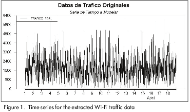
The Wi-Fi traffic series obtained for the 1,728 captured data can be seen in Figure 1.

Model identification

As one the objectives was to compare different correlated models (i.e. constructing different traffic models based on different time series and analyse which was the best one for estimating the captured Wi-Fi traffic), this identification stage made no sense for this research as, irrespective of model identification conclusions, four correlated traffic models were to be developed: an auto-regressive (AR) model, a moving average (MA) model, an auto-regressive moving average (ARMA) model and an auto-regressive integrated moving average (ARIMA) model. It is worth mentioning that the first three correlated models implied that the series needed to be stationary while there was no need for stationarity in the fourth model's time series (Brillinger, 2001).

The concept of stationarity is important when analysing time series. The random variables' joint density function must usually be known to fully characterise a stochastic process; however, in practice, it is not realistic to think that this can be achieved with a time series. As previously mentioned regarding covariance, there is no dependence on time but on separation (k) between variables. This led to thinking that the series would display the same general behaviour, irrespective of observation time. This meant that if a number of a series of contiguous observations were to be plotted, the graph obtained would be quite similar to the graph obtained when plotting the same number of contiguous observations but k periods forward or backward respecting the initially considered terms (Brillinger and Davis, 2002; Hamilton, 1994).

According to the above, the first three models (whose condition is series' stationarity) would not make sense in this case. The ARIMA model was thus the only one matching the time series and so the identification stage came to an end. However, as the aim was to compare the four models, the ARIMA model would be developed first because of its advantage of being "I" integrated, thereby allowing a non-stationary series to become stationary (following the trend). Once the ARIMA model was completed, the stationary trend was taken to estimate the AR and MA models (the ARI and IMA models, respectively). The ARMA model previously made nonsense because it led to the same ARIMA model after calculations were made (Box and Jenkins, 1976).

Parameter estimation and validation

1) The ARIMA Model. A Dickey-Fuller unit root test was carried out to verify time-series non-stationarity by using regression analysis of time series (RATS) software. The results obtained were as follows (Davis, 1996; Dickey and Fuller, 1979):

The series was non-stationary according to Dickey–Fuller criteria as the absolute test value was lower than the 5% critical absolute value. This arose from the fact that the data mean was not zero (Figure 1) although variance seemed to be constant. The series was differentiated to make it stationary and the unit root test was carried out again.

The original time series was used with its first 1,440 traffic data and was initially differentiated just once. It was then differentiated twice and the original time series logarithm was differentiated once. After these differentiations, each of the previously obtained series underwent the Dickey-Fuller Test to verify their respective stationarity.

It was thus concluded that the best transformation was a one-time series differentiation; it produced the series shown in Figure 2 (note that this time the data mean is zero).

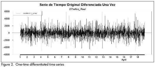
If only the first differences were applied, it was an ARIMA (p,1,q), if it required second differences, it was an ARIMA(p,2,q); in general, if (1-B)d was applied, an ARIMA(p, d, q) was obtained. Then, to develop this investigation d=1 (Brillinger, 2001).

Original series over-differentiation had to be prevented as well as the deletion of the valuable information that may arise from the auto-correlation function because in an over-differentiation case, auto-correlations become more complicated, the model loses parsimony, variance increases and d-observations are lost (Brockwell and Davis, 2002).

Having obtained a stationary series, the "p" order (auto-regressive) and the "q" order (moving average) had to be determined; auto-correlation function partial and auto-correlation function were used to do it (Akaike, 1973), (Anderson, 1980), (Davis, 1996).

Software RATS was used to obtain these auto-correlation and partial auto-correlation graphs (Figure 3). These two graphs (FAC and FACP) led to estimating the "p" and "q" values to construct the ARIMA (p,d,q) model we were interested in. Then, q=32 was obtained from FAC and p=32 was obtained from FACP. As the series was finally differentiated just once, then d=1. An initial ARIMA model was finally obtained (32,1,32).

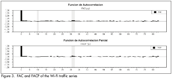
According to the FAC and FACP results, the model was represented by (1), but the coefficients were not yet known.

Now, having obtained a strong candidate, its parameters had to be estimated. In practice, this is a calculation task and a package must be selected to that end. Software RATS was selected for this study (rather than Eviews) because of its flexibility, great potentiality and maximum probability estimation.

It is usual to pass from initial estimation to residual analysis; however, peak points were being sought here among the residuals. Such peak points indicated the terms which had to be included in the ARIMA model's new formulation which would be estimated again. This dynamic respecification cycle is over when residuals show no more correlations (peaks); the residuals can then be deemed as white noise (Jones, 1978), (Makridakis, Wheeleright and Hyndman, 1997).

The model's parameters were first estimated with RATS software (i.e. the ARIMA model coefficients shown in (2)); their values are as follows:

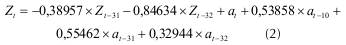
Figure 4 shows the model estimated via (2) based on time. Traffic data from a whole week was extracted to do this. However, it was not possible to validate the model from just simple inspection. Time series model validation is done by verifying the correlation between the model's residuals and this requires applying both the auto-correlation function (FAC) and partial auto-correlation function (FACP) to these residuals.

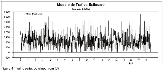
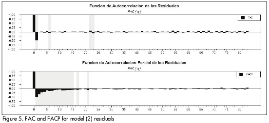
Figure 5 shows the FAC and FACP for the residuals from the model estimated in (2). Correlation can also be observed in this figure between the residuals from the (2) model; this model thus does not include the whole time series' dynamics. The model's coefficients had thus to be repeated and estimated again, now including the new values for "p" and "q" as suggested by the autocorrelation and partial auto-correlation functions, i.e. values 1, 2, 3, 4, 5, 6, 7, 8, 9, 10, 11, 12, 13, 14, 15, 17, and 21 for "p" and values 1, 6, 22 and 23 for "q". According to this, a new coefficient was estimated, including the new "p" and "q" parameters.

The previous procedure was carried out until the FAC and FACP residuals showed that there was no correlation between the estimated model residuals, this being achieved after 4 additional repetitions. The number of parameters obtained for the correspondding model was 21. A model having a large number of parameters does not show good parsimony. The significance level was thus analysed for each parameter and those above 5% were eliminated as they were not significant for the model. Having completed this part, the model had to be validated again and, depending on the result, repeated once more.

A definitive model was finally obtained as described by (3).

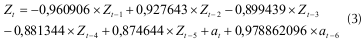
A six-parameter ARIMA model (5,1,6), as defined by (3), was finally obtained and a quantitative evaluation of this model was made (see section 3).

The same procedure was followed for the ARI and IMA models.

Results

Alternative models are usually found and one of them must be chosen. First, the auto-correlation function and the partial auto-correlation were applied to the final model's residuals to determine there was any correlation between them. If no correlation were found, then the model could be deemed to have been successfully validated. However, in this study no correlation was ascertained between the residuals from any of the three developed models and so the question was, "Which one should be chosen?" (Brillinger, 2001).

Other criteria were thus analysed besides the residual analysis so as to choose an appropriate model:

-Fitting quality criterion

-Parsimony criterion

-Statistic criteria

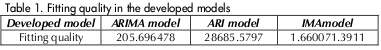
Fitting quality

A model fitting quality is defined as the sum of the residuals' squares divided by the sample size. Its object is to measure the model's capacity to reproduce the sample data (i.e. to verify how similar the modelled series and the actual series really are) (Guerrero, 2003).

Table 1 shows the fitting quality values for each developed model.

Parsimony

The idea of parsimony is that a good model has few parameters as it has captured the properties inherent to the analysed series; likewise, a complicated model with too many parameters is a model lacking parsimony. From this standpoint, the previously-obtained ARI model was a model lacking parsimony as it had a great amount of parameters (12 parameters in total) by contrast with the ARIMA (6 parameters in total) and IMA models (4 parameters).

It may be concluded that the IMA model showed the highest parsimony, even above that of the ARIMA model. However, it should always be the last criterion used to choose a model because of its qualitative rather than quantitative nature, as opposed to quality fitting criteria and those described below.

Statistical criteria

Even though an appropriate model may be selected from residual analysis, fitting quality and parsimony criteria, different statistical criteria were also calculated to allow making an objective comparative analysis between the developed time series models. The statistics calculated were:

-Mean square error

-Standard deviation absolute value

-Correlation coefficient

Standard deviation absolute values provided the most significant statistical value. Calculating the mean square error was decided on in this research as being average standard deviation from the square from the estimated values compared to the original data. All this was aimed at obtaining a quantitative value for the model's accuracy as the mean square error (by definition) would have the same value as the fitting quality criterion, which would not say how effective the model was; it only allows comparing it to others.

The standard deviation average for each estimated data was not significantly objective as it may assume positive or negative values thereby affecting the final results. It was thus decided to take the absolute value average for each data standard deviation.

The correlation factor between the estimated data and the original data was then calculated as these values provide an indication of the relational level between two variables, something the covariance function cannot achieve.

The results from abovementioned statistical criteria are shown in Table 2.

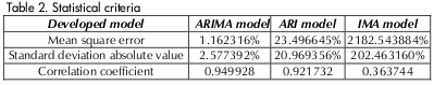
The ARIMA model was thus chosen as the best option for mo-delling the captured Wi-Fi traffic data from the results obtained for each criterion.

Evaluating prediction

In the real world, the thesis can be supported that a model is really only useful if it predicts variable evolution. One would thus wait for future observations to arrive before analysing a model's quality; this is called an expost evaluation and, regarding common sense, provides stronger validation than residual analysis.

288 traffic data were predicted for each model (288 = 1,728 – 1,440) and were respectively compared to the original traffic data. Table 3 shows prediction accuracy respecting statistics such as mean square error, the standard deviation absolute average value, correlation coefficient and quality fitting, allowing observing in detail how efficient each developed model was in predicting the respective traffic data.

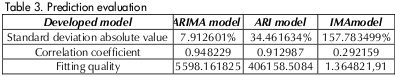
It was quite interesting to analyse the ARIMA model's prediction capacity as it had an average error of only 8% in traffic data predictions for the next three days, according to the standard deviation absolute value; however, how long will it maintain these amazing predictions for in the future?

Conclusions

The traffic series experienced stationarity in this Wi-Fi traffic modelling study because the demand patterns influencing the series were not relatively stable, thus requiring series transformation. This is generally done by differentiation (as done when developing the ARIMA model), again highlighting the significance of this modelling type. Time series, and especially ARIMA, are very appropriate for modelling modern traffic in Wi-Fi data networks having strong correlation characteristics. Evaluating the ARIMA model (developed and finally chosen as being the most appropriate in this study) showed a fairly high performance related to the residual dimension, which did not have any correlation.

Correlated models developed from time series do not experience a relationship as close as in the Poisson model and their mathematical management is compromised. However, they allow modelling Wi-Fi traffic with really significant precision and accuracy as they are able to capture correlation effects with reasonable computational efforts. This allows time series models to provide high performance when characterising Wi-Fi traffic (compared to the Poisson model) with computational effort which is as reasonable as the Poissonian model's mathematical management.

Bibliography

Akaike, H., Information theory and an extension of the maximum likelihood principle., Second international symposium on information theory, Budapest, 1973, pp. 267-281.        [ Links ]

Alzate, M. A., Modelos de tráfico en análisis y control de redes de comunicaciones., Revista de ingeniería de la Universidad Distrital Francisco José de Caldas, Bogotá, Vol. 9, No. 1, 2004, pp. 63-87.        [ Links ]

Anderson, T. W. Maximum likelihood estimation for vector auto-regressive moving-average models, directions in time series., Institute of mathematical statistics, 1980, pp. 80-111.        [ Links ]

Ansley, C. F., Kohn, R. On the estimation of ARIMA models with missing values., Time series analysis of irregularly observed data. Editorial Parzen, 1985, pp. 9-37.        [ Links ]

Box, G. E. P., Jenkins, G. M., Time series analysis: Forecasting and control., Revised Edition, Oakland, California: Editorial Holden-Day, 1976.        [ Links ]

Brillinger, D. R., Time series: data analysis and theory., Universidad de California, Holden-Day, SIAM, 2001.        [ Links ]

Brockwell, P. J., Davis, R. A., Introduction to time series and forecasting., Second edition, New York: Editorial Springer, 2002.        [ Links ]

Casilari, E., Reyes, A., Lecuona, A., Diaz, E. A., Sandoval, F., Caracterización de trafico de video y trafico Internet., Universidad de Malaga, Campus de Teatinos, Málaga, 2002.        [ Links ]

Casilari, E., Reyes, A., Lecuona, A., Diaz, E. A., Sandoval F., Modelado de trafico telemático., Universidad de Málaga, Campus de Teatinos, Malaga, 2003.        [ Links ]

Correa Moreno, E., Series de tiempo: conceptos básicos., Universidad Nacional de Colombia, Facultad de Ciencias, Departamento de matemáticas, Medellín, 2004.        [ Links ]

Davis, R. A., Maximum likelihood estimation for MA(1) processes with a root on or near the unit circle., In: Econometric theory, Vol. 12, 1996, pp. 1-29        [ Links ]

Dickey, D. A., Fuller, W. A., Distribution of the estimators for autoregressive time series with a unit root., J. Amer. stat. assoc. Vol. 74, 1979, pp. 427-431.        [ Links ]

Fillatre, L., Marakov, D., Vaton, S., Forecasting seasonal traffic flows., Computer Science Department, ENST Bretagne, Brest, Paris, 2003.        [ Links ]

Grossglausser, M., Bolot, J. C., On the relevance of long-range dependence in network traffic source., En: IEEE/ACM Trans., Networking 7, 1999.        [ Links ]

Guerrero, V. M., Análisis estadístico de series de tiempo económicas., Segunda edición, México: Editorial Thomson, 2003.        [ Links ]

Hamilton, J. D., Time series analysis., New Jersey: Princeton university press, 1994, pp. 25-152.        [ Links ]

Jones, R. H., Multivariate autoregression estimation using residuals., applied time series analysis, New York: Academic Press, 1978, pp. 139-162.        [ Links ]

Makridakis, S. G., Wheelwright, S. C., Hyndman, R. J., Forecasting: methods and applications., Tercera edición, USA: Editorial Wiley, 1997.        [ Links ]

Olexa, R., Implementing 802.11, 802.16, and 802.20 Wireless Networks: Planning, Troubleshooting, and Operations., Editorial Newnes, 2004.        [ Links ]

Pajouh, D., Methodology for traffic forescating., The French National Institute for Transport and Safety Research (INRETS), Arcuel, 2002.        [ Links ]

Papadopouli, M., Sheng, H., Raftopuulos, E., Ploumidis, M., Hernandez, F., Short-term traffic forecasting in a campus-wide wíreles network, 2004.        [ Links ]