The feasibility of daily, weekly and ten-day water-level forecasting in Colombia

Efraín Antonio Domínguez¹ Calle, Hector Angarita² and Hebert Rivera³

¹Hydrologist Engineer. PhD. Technical Sciences, Departamento de Ecología y Territorio, Facultad de Estudios Ambientales y Rurales, Pontificia Universidad Javeriana, Bogotá, Colombia. CeiBA – Complejidad, Bogotá, Colombia. ² Civil Engineer. M.Sc., in Hydrosystems, School of engineering, Pontifici Universidad Javeriana, Bogotá, Colombia. CeiBA – Complejidad, Bogotá, Colombia.³ Hydrologist Engineer. Ph.D., in Hydrology. Subdirección de Administración de los Recursos Naturales y Áreas Protegidas, CAR, Bogotá, Colombia.

Abstract

This paper analyses the feasibility of forecasting daily, weekly and ten-day water-levels at 20 hydrological stations forming part of the monitoring network supporting the Institute of Hydrology, Meteorology and Environmental Studies' (IDEAM) Alert Service in Colombia http://www.ideam.gov.co). Such viability was determined by a set of orthogonal performance criteria and implementing optimally adaptive linear combinations (OALC) was recommended for this study as a viable operator for configuring a real-time hydrological forecast system. It is shown that the forecast for daily, weekly and ten-day levels had satisfactory viability for 70% of the cases studied.

Key words: Hydrological forecasting, mathematical modelling, optimal linear adaptive combination.

Received: may 18th 2009

Accepted: jun 21th 2010

Introduction

Hydrological forecasting is one of the most important facets of hydrology. The feasibility of conducting real-time hydrological forecasting is a feature of modern times that appeared with the beginnings of scientific hydrology seated in 1674 by Pierre Perrault (Perrault, 1674). Observation of the weather and the state of surface runoff and other water sources dates from the Egyptians in the Nile valley (www.waterhistory.org/histories/cairo/). However, only until the establishment of systematic and standardised measurement did it become possible to think about a hydrological warning system setup. Colombia has not been far from the international trend that issued guidelines for establishing monitoring networks for water resources and early warning systems which would help take advantage of real-time hydrological information and its combination with advances in computers and the media. The Colombian Hydrological and Meteorological Service (CHMS) dabbled in hydrological forecasting with the Sacramento model in 1976; this was operated by punch cards and assimilating information transmitted by radio and telephone.

The system emitted quantitative predictions and supported disaster-preventing agencies in managing season floods during winter. Colombia has no hydrological models for real-time quantitative hydrological forecasting today, even with the increased availability of technology in computing and telecommunications fields. IDEAM has made efforts to implement a quantitative real-time hydrologic forecasting service aimed at restoring institutional capacity in hydrological forecasting.

This paper examines IDEAM's institutional capacity (strengths and weaknesses) for undertaking operational quantitative forecasts for daily, weekly and ten-day frameworks. The feasibility of quantitative, real-time hydrologic forecasting is defined here, being set by studying aspects such as staff training level, computational capacity, continuous hydrological records (real-time hydrometrical network), the availability of software for integrating hydrometeorological information flows and the quality of real-time information. The final stage gives a detailed analysis of the possibility of issuing real-time hydrological forecasting based on a mathematical technique providing operators with endogenous (auto-regressive) and exogenous components and also has an explicit optimisation mechanism. The viability of forecasts raised here is conceived through completeness in infrastructure and staff and the possibility of having a mathematical structure optimised according to selected performance criterion. A work plan is presented for achieving concrete real-time forecast of daily, weekly and ten-day average water-levels.

Methods and data

This study was developed through four methodological steps: reviewing previous quantitative modelling for hydrological forecasting in IDEAM, defining hydrological forecasting feasibility, applying optimally-adapted linear combinations (OALC) for daily, weekly and ten-day water-level forecasting at IDEAM's hydrological warning system's stations and defining criteria for scoring the feasibility of a forecast at a given hydrological station and for all forecasting stations. Hydrometeorological information used was obtained from the IDEAM database which stores real-time information on rainfall and water-levels. The analysed forecast points are presented in Table 1. Time-series obtained from the IDEAM database from stations which do not operate in real-time were also used in some cases. The latter are used as forecast predictors in the stations for which no predictors were found amongst stations transmitting real-time information.

Review of quantitative modelling for water in IDEAM forecasts

Quantitative forecasting of water-levels is one of the priority goals for IDEAM's hydrological warning system. Several investigations have been carried out for implementing quantitative forecasts, ranging from qualitative models based on semantic and fuzzy logic rules (Rivera et al., 2004), time-series technique (Mussy, 2005), to advanced models capable of predicting the probability density

curve for daily levels of data itself rather than water-level (Domínguez, 2004a, Domínguez, 2004b; Domínguez, 2005). These have had the following difficulties. They have not been done in coordination and have also lacked common performance criteria for measuring comparative advantages amongst different forecast operators. There has thus been no standard for documenting the models proposed, characterising input, output, operators, state variables, parameters and calibration procedure. There has been a characteristic lack of standardisation regarding forecast horizons, date ranges for calibration and validation and defining rules establishing thresholds for accurate forecasting.

Defining the feasibility of hydrological forecasting

A quantitative hydrological forecasting system can become operational and viable when (WMO, 1994) the following conditions have been met: The necessary infrastructure for real-time water-level measurement and transmission exists; There is available detailed physiographic, hydrological, meteorological and topographic information regarding the points where the forecast is emitted; Trained staff are available for analysing the assimilated real-time hydrological information, as well as operating the hydrological forecasting models and computational infrastructure needed to run these models; There is forecasting technology for making real-time predictions, having acceptable performance levels; There are formalised channels for broadcasting hydrological forecasting; and An officially registered user community has been established and is able to assimilate the forecasts issued and provide feedback for the hydrological warning system. Analysing IDEAM's measurement infrastructure, telecommunications and staff it was concluded that IDEAM's hydrological warning system completely failed to fulfil requirement (d) and partially with condition (f). A real-time forecasting technique is thus proposed which is suitable for the flow of information currently available in IDEAM's hydrological warning system.

Optimally adaptive linear combinations (OALC) for daily, weekly and ten-day water-level forecasts in IDEAM's hydrological warning system's stations

An important element in the emission of hydrological forecasts is the availability of a mathematical operator <L> using real or near-real-time predictors for forecasting the future state of levels for a forecast horizon T. There is a wide range of operators available for that purpose, from the simple to the most complex. Examples of hydrological forecasting mathematical operators would include: Mathematical models in ordinary differential equations (Kovalenko, 1993; Kuchment, 1972b), Mathematical models of partial differential equations for describing hydraulic transit in one and two dimensions (Kuchment, 1972a; Rudkivi, 1979, WMO, 1975); Mathematical models in stochastic differential equations (Gardiner, 1985; Kovalenko, 1993), Models based on the theory of optimal Kolmogorov extra / interpolation (Kolmogorov, 1941); Auto-regressive and regressive methods (Kazakievich, 1989; Popov, 1957, WMO, 1994), Statistical models (Haan, 2002; Rozhdientsvienstkiy and Chievatariov, 1974); Fuzzy logic-based models (Ashu and Avadhnam, 2007; Luchetta and Manetti, 2003); and Neural network-based models (Ashu and Avadhnam, 2007; Luchetta and Manetti, 2003).

These models can be classified as proposed by Domínguez (Domínguez, 2007) so that they can generally be differentiated by their ability to represent static or dynamic processes, lumped or distributed systems, deterministic or stochastic relationships. The range of possibilities is diverse, so some minimum requirements for operator L, had to be established. In fact:(a) L must meet the stated objectives of the hydrological warning system and fulfil forecast users' expectations;(b) It should be as simple as possible in its use by forecasters: the algorithm implementation source code should be explicit enough for operation by staff; (c) It should be consistent with the available computing power and precision levels of the predictors recorded in real-time,(d) It should have an operating optimisation algorithm which must be dynamic and adaptable to water-level data coming in in real-time and adjustable during the event of loss of reception of one of the predictor signals; and (e) It should be applicable to different physiographic conditions of forecast points.

Based on these characteristics, and according to Kazakievich (1989), any differential equation can be reduced to the form of regression or auto-regressive model, including partial differential equations (Zwillinger, 1997). A technique for modelling and forecasting based on adaptive optimal operators is given below. This technique provides optimal forecast operators in a linear space and defines the optimal parameterisation window through exhaustive search requiring minimum computational times, making it suitable as a forecasting tool in real-time early-warning systems.

Usually a mathematical modeller calibrates a mathematical mode's parameters, trying to use the maximum available historical information. Here, this paradigm has been contradicted by showing that a dynamic calibration of linear combinations can yield a more efficient mathematical operator than that in which the coefficients take static values obtained from information from the entire time-series for the variable being predicted. This can be particularly useful when the recorded time-series exhibit different scale and frequency oscillations and for which prediction is aimed for a lead time no higher than T≤ ρ with ;ρ << Ns where «T» represents the forecast horizon, ρ the process auto-correlation radius and Ns is the total length of the time series of the variable being predicted.

Given a time interval [t-N-1,t]∈ℜ in which N was record length, then forecast Y(t+T) could be expressed as follows:

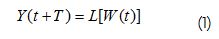
In (1) L is a mathematical operator working on a polynomial W(t) of order k=max(α_i ;β_j ) using endogenous and "m" exogenous predictors in the form (Kolmogorov, 1941):

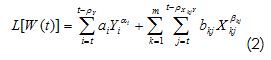
Where ρ_Y and ρ_XkjY were the radius of autocorrelation of the endogenous variable ρ_{X kjY} and the radius of cross-correlation between the last and the exogenous variable X(t)_k . In turn, a_i, b_bj,a_i and b_kj were the coefficients and exponents in polynomial W(t).

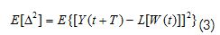
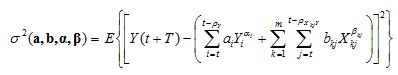
If the difference between Y(t+T)^Observado - Y(t-T)^Pronosticado= Δ , L could be referred to as an optimal operator if it minimised some function of Δ , for example the expected value of the square mean error:

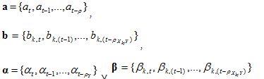
When a finite vector of values taken by Y(t) was known and if its correlation radius was equal to ρ_y, then forecast valueY(t+T) could be represented as a combination of values Y(t) and the exogenous variable X(t) taken from t until t-ρ_Y for Y(t) and from t to t-ρ_Y so that:

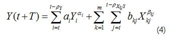
where a_i, b_i,a_i and b_i were the coefficients and exponents that minimised:

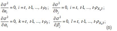
In a time window of length θ. That stated above would result in the aforementioned domain

being solutions for the following system of equations

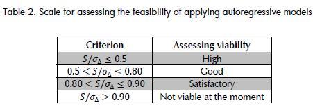
For a time interval of length θ it might also be required (even for non-linear combinations) that the relationship between ,– the deviation from the mean square error of forecasts and σΔ, the standard deviation of increments of Y(t) for lead time «T» to be less than or equal to 0.8, requiring an a-priori compliance of performance criterion S/σΔ as used in Domínguez (Domínguez, 2004a). Other performance criteria which can be used as objective function have been presented by Dawson (Dawson et al., 2007). However, it is advisable to define a set of performance criteria as being orthogonal. Therefore, criterion S/σΔ, the percentage of accurate forecasts, the standard square error and the coefficient of determination between observed and simulated data as such set have been used for this study.

Selecting predictors

Endogenous variable Y(t) and exogenous, for example Xi(t), delayed in t – mΔt, where m=0… ρ with ρ characteristic cross-correlation radius for each predictor could be postulated as predictors. It was advisable that the cross-correlation matrix between selected predictors and the variable to be predicted should be constructed to get an overview of the forest and not just the trees. Henceforth,the following was considered:

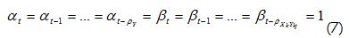
This reduced the search for optimal operator to a space of first-order polynomials. Predictors having coefficients {a_t,a_t-1,...,a_t-ρ} and {b_t,b_t-1,...,b_t-ρY} , satisfying constrains (a_k/σ_ak≥2)or (b_k/σ_bk≥2), had to be chosen to filter the predictors and only use those that provided non-redundant information. To be precise, only coefficients a_kor b_k greater than twice the standard definition square error of the coefficient (σ_ak or σ_bk) were used. As exogenous predictors, in the case of hydrological forecasts, current and lagged rainfall information and the information on river inflows may be used. An exhaustive search algorithm is usually able to establish the optimal number of predictors amongst all available combinations using criterion S/σΔ as objective function. The minimisation of the function presented in equation (5) may be advanced by the least squares method, the conjugate gradient or even by bio-inspired techniques (Yang et al., 2003; Боглаев, 1990). Examples of the power of the conjugate gradient method can be found in Press (Press et al., 1986) and Fylstra (Fylstra et al., 1998). Other analysis conducted to establish the optimal number of predictors could be by determining the number of independent observations and error equivalently corrected coefficient of multiple determination, evaluating the evolution of criterion S/σΔ and evaluating the level of informativeness for each predictor group and constructing ion the saturation function. The number of equivalently independent observations m₁ determined as:

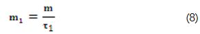
Where the radius of autocorrelation τ₁ was thus defined as:

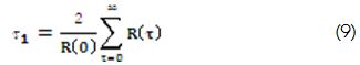
Here R(τ) was the autocorrelation function and R(0) its maximum value. Thus, the error of the coefficient of determination Δ_R taking into account the number of equivalently independent observations, was:

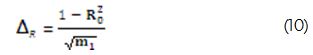
The optimal group of predictors was thus chosen as being the group that minimised the standard error for the coefficient of determination (State Hydrometeorological Committee of the USSR, 1989). Another way to choose the best predictors' group was by evaluating the level of informativeness of predictors separately and in different sets of predictors. The best group of predictors was formed by the minimum number of those achieving saturation point in the saturation function. The saturation function was constructed as being the level of informativeness for the predictors' groups with a different number of predictor variables in the group. The level of informativeness was defined as being:

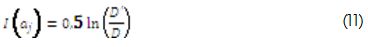
Where D was the determinant of the correlation matrix between water-level values and their predictors and D';was the determinant of the predictors' correlation matrix. I(a_j ) represented the informativeness for a group of j predictors (State Hydrometeorological Committee of the USSR, 1989).

Classification criterion for forecast feasibility assessment at each forecast point and for a set of hydrological stations

Different forecast feasibility levels were established for assessing the viability of predicting daily, weekly and ten-day averaged water-levels in terms of S/σΔ criterion and taking care of the percentage of successful forecasts using the maximum permitted error (MPE) as threshold. It also took into account whether the information from the predictors could be found online at the time of issuing the forecast. Table 2. gives the results of S/σΔ criterion forecasting viability. The number of successful forecasts given a maximum permitted error is appended to the feasibility reading. One outcome might have been that the forecasting procedure was viable (70% successfulness) given 15% MPE (mean absolute error). This appendix does not affect the conclusion about the feasibility of implementing optimal adaptive operators for predicting water-levels, since IDEAM forecast users' requirements remain unknown. Moreover, the natural process predictability must also be taken into account when setting the maximum error allowed for setting the level of correct forecasts point. The maximum permissible error, according to the natural variability of the process, was set to ( Апполов et al., 1974): MPE = 0.674 σ_Δ.

Results

More than 300 numerical coarse-tuning experiments were conducted on forecasting feasibility for daily, weekly, and ten-day average levels. Smaller sets of predictors were present in each experiment. Each experiment represented a search from 540 possible combinations for each case (i.e. a total of 162,000 coarse optimisation tests were made). Such optimisation was unsupervised and took an average 4 hours computation time on a dual-core processor computer having 2.33 GHz frequency and two GB of RAM. No parallelisation algorithms were used (vectorisation) so specified times were subject to reduction. After the coarse-tuning, 20 experiments were then conducted to refine the set of optimal predictors. Such optimisation was supervised and was performed semi-automatically. Each optimisation exercise reviewed groups of three predictors which could be assembled into a set of 10 potential predictors by taking into account the autoregressive components and cross-correlation lags. In theory this requires reviewing 120 possible combinations; however, following the recommendations given in the predictor selection paragraph, this number was drastically reduced to about 10-20 combinations. The tuning exercise for the 20 selected stations reviewed about 400 combinations. On average, per station, about 15 minutes was spent in tuning, thereby adding 5 hours to setting up the forecast for all stations.

Taking an information integration platform and trained forecasters, this computational time could become reduced by half; however, if it were required to set up an operative forecast system, these tasks could not be performed by a single person. As a minimum, it would be expected that a staff of two trained forecasters should be used. The times presented here were valid for all 20 stations selected here. A larger set of stations would require more time; however, a parallel computing approach would be desirable.

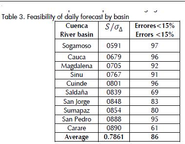
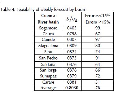
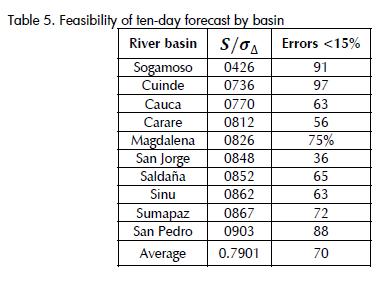
It can thus be concluded that the feasibility of prediction decreased by increasing the aggregation period (i.e. the best predictability of levels was obtained on daily data and the worst on ten-day averaged data). This view was supported by the magnitude of criterion S/σ_Δ which was 0.740 on average, for all 20 stations, on a daily basis, while being 0.803 and 0.797 at weekly and ten-day aggregations, respectively. In turn, the percentage of successful forecasts according to maximum permitted error was 81.5% for a ten-day averaged water-level forecast, 82.9% for a weekly one and 86.5% for daily water-level forecasts. The percentage of success with errors less than 15% was 89.9% for daily, 75.7% for weekly and 70.3% for the ten-day forecasts. The feasibility of implementing OALC operators was good for the different types of forecasts if the results were sorted by aggregation level, basins having improved feasibility for implementing such operators for forecasting daily levels would be those for the Sogamoso, Cauca, Magdalena and Sinu rivers and the worse would be for the San Pedro and Carare rivers in which only a satisfactory rating of viability was achieved. In the field of weekly forecasting the best feasibility rate was reached by the Sogamoso River, while the Carare river retained the lowest viability (satisfactory according to the scale shown in Table 2). In the case of ten-day forecasts, the Sogamoso, Cuinde and Cauca rivers remained as being the most predictable and the San Pedro river was ranked as having the lowest predictability. A 77% level of successfulness was reached for all forecast types from the standpoint of the number of successful forecasts having a 15% MPE. This fact reinforces the conclusion regarding the feasibility of implementing adaptive operators for real-time forecasting of water-levels using information from IDEAM's real-time hydrological network.

Conclusions

The feasibility of forecasting daily, weekly and ten-day averaged water-levels at the nodes of IDEAM's real-time hydrological network was good. Over 70% of the analysed hydrological stations reported S/σ_Δ ;≤0.85 performance values and 70% successfulness for a 15% MPE.

The forecasting technique analysed for both computational time and forecast error offered good performance for the different aggregations. The proposed forecasting methodology led to determining which hydrological stations should be upgraded and included in the real-time transmission system. For specific cases in which the viability of forecast was not satisfactory there is still space for improvement by including predictors which were not considered here.