Andrés Pantoja¹ , Eduardo Mojica Nava² y Nicanor Quijano³

¹ Electronic Engineering, Universidad Nacional de Colombia Sede Manizales. M.Sc., in Electronic Engineering, Universidad de los Andes. Ph. D., Student, Universidad de los Andes. Universidad de Nariño, Pasto. ad.pantoja24@uniandes.edu.co

²Electronic Engineering, Universidad Industrial de Santander. M.Sc., in Electronic Engineering, Universidad de los Andes. Ph.D., in Engineering, Universidad de los Andes y Ecole Centrale Nantes, Francia. Universidad Católica, Bogotá, Colombia. ea.mojica70@uniandes.edu.co

³Electrical Engineer, Pontificia Universidad Javeriana, Bogotá, Colombia. M.Sc.,and Ph.D., in Electronic Engineering, Ohio State University, Columbus, OH,USA. Universidad de los Andes, Bogotá, Colombia. nquijano@uniandes.edu.co

ABSTRACT

The sum of squares (SOS) decomposition technique allows numerical methods such as semidefinite programming to be used for proving the positivity of multivariable polynomial functions. It is well known that it is not an easy task to find Lyapunov functions for stability analysis of nonlinear systems. An algorithmic tool is used in this work for solving this problem. This approach is presented as SOS programming and solutions were obtained with a Matlab toolbox. Simple examples of SOS concepts, stability analysis for nonlinear polynomial and rational systems with uncertainties in parameters are presented to show the use of this tool. Besides these approaches, an alternative stability analysis for switched systems using a polynomial approach is also presented.

Keywords: sum of squares (SOS), stability analysis, nonlinear systems, switched systems.

Received: april 30th 2009

Accepted: november 15th 2010

Introduction

The theory of sum of squares (SOS) decomposition of polynomial functions has achieved significant progress during the last ten years since its introduction (Parrilo, 2000). This development has resulted from possible relaxations of NP-hard problems (e.g., non-negativity proofs of multivariable polynomials) (Papadimitriou, 1994) for solvable problems in computational polynomial time. The basic problem consists of finding conditions to verify. The possible classes of F functions must be limited to study this problem from an algorithmic approach and, at the same time, to keep the problem general enough to guarantee the applicability of the results. A tradeoff is achieved when the class of F functions is restricted to polynomial functions (Parrilo, 2000)

Definition 1.1. A polynomial function f in x₁, . . . , x_n, with coefficients in a field k, is a finite lineal combination of monomials:

f= ∑_αc_αx^α=∑_αc_αx₁^α1...x_n^αn c_α>k (2)

where the sum is given over a finite number of n -− tuples

α = (α₁, ..., α_n), con α_i∈ N₀.

It is possible to show that proving polynomial function global positivit is in fact an NP-hard problem too (when the degree of the function is at least four). Therefore, a method guaranteeing the solution of this problem for any polynomial function could have unacceptable computational performance for a function having a high number of variables. This is the main disadvantage of theoretical methods so that the quantifiers are eliminated (Parrilo, 2000).

A question arises when inherent computational complexity problems must be avoided. Do some conditions guarantee the positivity of a multivariable function so that the method can be executed in polynomial time? The next section shows that SOS descomposition techniques fulfil complexity reduction conditions.

Some SOS technique applications are global, boolean and constrained optimization problems (Prajna et al., 2004). Moreover, some general control problems, such as Lyapunov's function construction for stability analysis of nonlinear systems (Topcu et al.,2008) and parameter uncertainty limitation in dynamic system analysis (Topcu and Packard, 2009) have been solved using the SOS approach. Other specific control applications are stability analysis of nonlinear systems with time delay (Papachristodoulou, 2004) and the synthesis and design of nonlinear controllers (Franze et al., 2009; Ebenbauer and Allg¨ower, 2006).

SOS techniques solve a convex optimisation problem by means of semidefinite programming (SDP) (Parrilo, 2003). This method is a generalisation of linear programming (LP) where non-negativity constraints in decision variables are replaced by positive semidefinite matrix inequalities. The methods for solving SDP are given by algorithmic techniques such as linear matrix inequalities (LMI) and numerical programmes for SDP such as SeDuMi and SPDT3 (Anjos and Burer, 2007).

Solving an SOS problem implies SDP problem construction, finding the numerical solution, and interpreting the result of the SDP problem in initial variable formulation. The Matlab toolbox SOSTOOLS (Prajna et al.,) was used for defining SOS variables,functions and constraints needed for resolving the optimisation problem in a symbolic environment.

This tutorial presents and reviews the basic concepts of SOS techniques and some control applications such as Lyapunov function construction for stability analysis of nonlinear systems, parameter uncertainty analysis in systems having rational vector fields, application in stability analysis of switching systems and the use of SOSTOOLS for solving some problems and examples.

Sum of squares (SOS)

The main concepts and basic examples of SOS techniques are presented in this section. As stated, these concepts were originally introduced by P. Parrilo (Parrilo, 2000). The examples start with SOS decomposition of a multivariable polynomial function to introduce some control applications.

The Matlab toolbox SOSTOOLS is introduced as a computational method used in the numerical solution of SOS problems introduced in this tutorial.

Basic concepts

Definition 2.1. A multivariable polynomial p(x) having degree 2d in x ∈ Rⁿ, is a sum of squares (SOS) if there exists M polynomials f_i(x) so that

p(x)= ∑_i=1^M f₁²(x)            (3)

SOS decomposition can be expressed as shown by Parrilo (2003) if there is a positive semidefinite matrix Q ∈ R^n×n, so that

p(x)=Z(x)^T QZ(x)        (4)

where Z(x) is a vector of monomials in x with a degree less than or equal to d. Given that Q = Q,^T _ 0 can be written as Q = HH^T, where H ∈ R^n×r with r = rank(Q), and if h₁, h₂, . . . , h_r, are the columns of H, then equation (4) can be expressed as

p(x)= ∑_i=1 (h^T₁Z(x))² (5)

Therefore, SOS decomposition can be relaxed to find matrix Q _ 0 and the resulting problem becomes a semidefinite programming issue as defined by Parrilo (2000).

The next example presents the representation of a polynomial function in an SOS form expressed as in equations (4) and (5).

Example 2.1. Find SOS decomposition of the polynomial function given by

p(x) = 13x⁴₁+14x³₁x₂-18x²₁+14x²₁x²₂...

With a vector

Z(x) = [1 x₂² x₁x₂ x₁²]^T 

a matrix Q^T≥ 0 is found so that

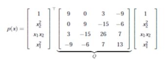
Then, with factorisation Q =HH^T  given by

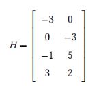
The resulting SOS decomposition is

p(x)= (3x₁²-x₁x₂-3)² + (2x²1-3x²2+5x₁x₂)²

Clearly an SOS function is globally positive, but not all positive functions are SOS.

An example of these functions would be the Motzkin polynomial M(x) = x⁴₁ x²₂+x²1x⁴₂+x⁶₃−3x²₁x²₂x²₃. To prove positivity in this class of functions using SOS techniques, Reznick (2000) has shown that if p(x) > 0, for all x ∈ Rⁿ, then there exists a positive integer r so that

     p(x)(∑ⁿ_i=1x²₁)^r       is SOS

The non-negativity problem is relaxed for testing different values of r until SOS representation is possible.

SOSTOOLS computational tool

SOSTOOLS (Prajna et al.,) is a Matlab toolbox which is used to solve SOS problems with an algorithm for semidefinite programming(e.g., SeDuMi or SDPT3).This tool turns the SOS problem into an SDP problem, uses the solving algorithm and expresses the solution in the initial variables and polynomials. The general procedure for obtaining SOS problem solution using SOSTOOLS is summaryzed as follows:

- Define SOS variables, polynomials and constants using the symbolic toolbox, or in Matlab polynomial format;

- Define the problem's constraints as SOS inequalities; and

- Use the SOSTOOLS functions for solving the problem and for expressing the solution in the problem's initial variables.

The next section presents some control applications which use SOS techniques to obtain a Lyapunov function which can be used for the stability analysis of the equilibrium point for nonlinear and switched systems

Control applications

Finding a Lyapunov function to prove the stability of an equilibrium point in a nonlinear system is a difficult task, except for systems having few variables and special vector fields (e.g., energy functions and gradient systems), where specific methods (e.g., Krasovskii) could be used (Khalil, 2002).

For more general systems, SOS techniques facilitate finding an appropriate Lyapunov function using a computational tool and fixed algorithm. The conditions for verifying the stability of an equilibrium point in systems having polynomial and rational vector fields rely on non-negative functions which could result in NPHard problems. Therefore, by turning these conditions into SOS functions, the problem can be solved using the SOSTOOLS computational tool.The tool is applied to polynomial and rational systems having parameter uncertainties in the next examples using variations of the simple original algorithms and extensions of the fundamental theorems in Lyapunov analysis.

Systems having polynomial and rational vector fields

The Lyapunov stability theorem is applied to the general autonomous system given by

          x^.=f(x)        (6)

where f : D →Rⁿ is a continuous map from D ⊂ Rⁿen Rⁿ, and without loss of generality (Khalil, 2002), the origin is an equilibrium point of (6) (i.e., f (0) = 0). If a continuously differentiable function V(x) (so-called Lyapunov function) is found, the system's stability conditions are defined by: i) if V(x) is positive definite, and ii) V(x) is negative semidefinite, the origin of (6) is stable; and ii) if V(x) is negative definite, the origin is asymptotically stable.

This theorem's conditions must be relaxed to apply the SOS techniques for proving stability in nonlinear systems to express non-negativity as SOS. In polynomial systems having state variables x = [x₁, x₂, . . . , x_n], a function V(x) with degree 2d is defined using an auxiliary function φ(x) given by

φ(x)= ∑_i=1ⁿ ∑ⁿ_j=1ε_ijx₁^2j (7)

where e ε ≥ 0, for all i and j, and ∑^a_j=1ε_{ij> 0}, for alli = 1,2, . . . ,n. With these conditions, j(x) is positive definite. Therefore, if V(x)−φ(x) can be expressed as SOS, it is guaranteed that V(x) is positive definite too. Stability conditions can then be expressed as:

V(x)−φ(x) es SOS (8)

- ^δV/_δx f(x) es SOS (9)

Hence, the SOS algorithm for finding a Lyapunov function using SOSTOOLS is stated as follows:

- Define a general polynomial function V(x) with degree 2d and monomials in x with degree d;

- Create the auxiliary function φ(x) as defined in (7);

- Define the expression V(x)−φ(x) as SOS. Inequality;

- Define - ^δV/_δx f (x) as SOS inequality; and

- Solve the SOSTOOLS programme and obtain the resulting V(x).

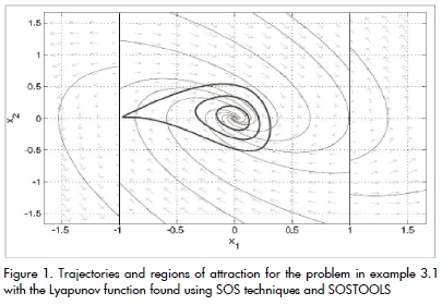
Example 3.1. (Khalil, 2002). Find a Lyapunov function to show asymptotical stability of the origin in the system:

x^.₁= x₂(1-x²₁)

The system has an equilibrium point in x = 0. This equilibrium is not the only one, given that in x₁ = 1 y en x₁=−1, x₁=0 and x₂=0. Then, finding a Lyapunov function that satisfies conditions (8) and (9) is not an easy task for analysing the origin's characterristics. Moreover, a region of attraction can be determined using the contour lines of the function V(x) so obtained.

Using SOSTOOLS, a function having 42 terms and degree 8 is found. Figure 1 shows the system's phase plane and the contour lines of V(x). It is shown that the biggest region of attraction is obtained when the contour lines approximate to x₁ = −1, which is thelimit where the isoclines of the Lyapunov function are closed.

In a system having a rational vector field f (x), condition (9) is modified to apply the SOSTOOLS algorithm. In this case, a function w(x) > 0 must be found so that

-w(x)- ^δV/_δx f(x) sea SOS and polynomial           (11)

If w(x) > 0, the second condition of the general stability theorem is satisfied, and if (11) is a polynomial function, the SOS techniques can be applied as shown in the next example.

Example 3.2. (Khalil, 2002). Find a polynomial Lyapunov function to show stability of the origin of the system given by

x^.₂= -2(x₁+x₂)/(1+x₁2)²        (12)

Choosing w(x) = (1+x²₁)² ≥ 0, and given that V(x) is a polynomial function, the algorithm for finding the Lyapunov function must include −(1+x₁2)^{2 δV}/_δx f (x) as SOS inequality to satisfy the second condition of the stability theorem.

The result of this SOSTOOLS programme is a function V(x) with 62 terms and degree 10. The phase plane and some contour lines of V(x) (i.e., regions of attraction of the origin) are shown in Figure 2.

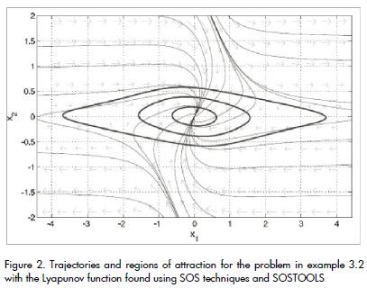
The system in (12) has a unique equilibrium point in x = 0, and the Lyapunov function obtained leads to establishing regions of attraction for the origin.

Although the Lyapunov functions found in examples 3.1 and 3.2 have a high number of terms, these functions are in the Matlab symbolic environment which facilitates plotting and verifying stability conditions.

Besides, the examples presented here have given a glimpse of the use of SOS techniques for analysing more complex and higher order systems.

Systems with parameter uncertainties

Consider the general nonlinear system given by equation (6) with parameter uncertainties expressed as

c_i(x,u)≤0 para i=1,...,N₁          (13)

where u ∈R^m is the set of uncertain parameters, and N₁ is the number of required constraints.

Assume that functions ci can be expressed as polynomial functions in (x,u), and that f (x,u) is a rational or polynomial vector field in (x,u) without singularities in D ⊂ R^n×m, where D = {(x,u) ∈ R^n×m|c_i(x,u) ≤ 0, for all i. Without loss of generality, it is assumed that f (x,u)= 0 for x = 0 and u ∈ D⁰ u , donde D⁰ u = {u ∈ R^m|(0,u) ∈ D}.The following theorem taken from Papachristodoulou and Prajna (2002) gives us the conditions for local stability of the origin of the system (6) constrained by (13).

Theorem 3.1. Suppose that for the system described above, there are polynomial functions V(x), w(x,u), and pi(x,u) so that: V(x) is positive definite in a neighbourhood of the origin, w(x,u) > 0 and pi(x,u) ≥ 0 in W Then, if

it guarantees that the origin of the state space is a stable equilibrium of the system (6). In the case where f (x,u) is a rational vector field, a function w(x,u) > 0 must be chosen so that −w(x,u)^δV/_δx f(x,u) is a polynomial function, and SOS algorithm can be applied without additional modifications. These conditions can be relaxed to SOS definitions according to the following proposition taken from Papachristodoulou and Prajna (2002).

Proposition 3.2. For a polynomial function φ(x) ≥ 0 (or SOS) defined as in equation (7), the local stability of the origin of (6) can be guaranteed if:

V(x)−φ(x) is SOS (i.e., V(x) is positive definite). Z(x,u) is SOS.

p_i(x,u), is SOS, for i = 1, . . . , N₁.

Using this proposition, the algorithm to find the Lyapunov function preserves the first three steps used in systems without constraints. The differences for systems with parameter uncertainties are defined for the condition given by (14). The next steps are required for this definition:

- Define a number of SOS functions pi(x,u) equal to the number of inequality constraints in the problem;

- Choose a function w(x,u) > 0 if necessary for a rational vector field f (x,u);

- Define −w(x,u)^δV/_δx f(x,u) + ∑ p_i(x,u)c_i(x,u) as SOS inequality; and

- Solve the SOSTOOLS problem and obtain V(x).

The next example applies the previously described procedure for evaluating the stability of the equilibrium point in a multi-zone thermal system with a controller based on evolutionary game theory (Pantoja and Quijano, 2008).

Example 3.3. A system with multiple disjoint temperature zones can be modelled by

T_i=-a_iT_i+b_ix_i+a_iT_a

where Ti is the temperature in the i^th zone (i = 1, . . . ,N), a_i,b_i are positive constants, T_a is ambient temperature and xi is control input for zone i. Assuming that B is a temperature limit so that B >> T_a, and with variable change qi = B−T_i the system can be expressed by:

q_i^.= -a_iqi-b_ix_i+a_i(B-T_a)       (15)

The control signal dynamics are designed so that the temperature in all zones achieves an equilibrium point equal to the maximum uniform temperature that can be obtained with a limited amount of power resources. The control strategy is given by the replicator dynamics concept (Pantoja and Quijano, 2008):

x₁^.= x₁ (q₁-1/P∑_j=1^Nx_jq_j)     (16)

where P > 0 is the total available amount of resources for heating all zones. Then ∑_j=1^Nx_i= P. The equilibrium point of the complete system composed by equations(15) and (16) is:

x*₁=^aj/_bjP/∑_j=1^{N aj}/_bj

q*₁= (B-Ta)- P/∑_j=1^{N aj}/_bj

The final temperature in each zone is given by:

T₁*= T_a+P/∑_j=1^{N aj}/_bj, para i =1, ...,N

which is clearly constant and depends on the system's parameters and on the available resources.

The proposed problem is to analyze the stability of the equilibrium point, given limited variations in the parameters of each zone a_i and bi for a two-zone system (i.e., N = 2).

To express the system in "error coordinates" so that the equilibrium point is displaced to the origin, the displacement variables are eqi = q_i−q*_iy e_xi= x_i−x*_i. Taking into account that x₁ + x₂ = P, x*₂ = P−x*₁,, then e_x2 = −e_x1. With these conditions, the system is given by:

e^.₁= (e_x1+Pa₁b₂/a₁b₂+a₂b₁)(e_q2-e_q1)...

(a₁b₂/a₁b₂+a₂b₁ + e_x1/_P -1)

e^._q2= -a₂e_q2+b₂e_x1

and the origin is the unique equilibrium point.

Appropriate estimated ranges for the parameters' variations are:

0 < a_i< 2 para i = 1,2

0 < b_i < 0,01 para i = 1,2

These inequalities must be expressed in polynomial form to be included in the SOS algorithm. For this purpose, if we assume that a and a are the lower and higher limits for a, respectively, inequality a < a < a is expressed as (a−a) (a−a) < 0. Defining polynomials p_i(x,u), for i = 1,2 as SOS variables, and w(x,u) = (a₁b₂+a₂b₁)² > 0, condition (14) is implemented as SOS inequality in the SOSTOOLS algorithm.

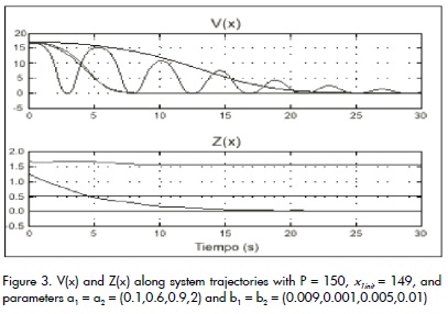
The resulting V(x) is a Lyapunov function with 32 terms and 4 degrees whose trajectories throughout the system's solutions are shown in Figure 3 for different parameter values within the specified ranges, with P = 150, and initial condition x₁ = 149. Moreover, this Figure presents the trajectories of Z(x,u) for the same conditions.

It is interesting to notice that V(x) and Z(x,u) just need to be positive to satisfy the conditions in Theorem 3.1. Near the fixed limits of uncertainty, the functions are close to zero, showing the activation of the constraints and the need for finding another Lyapunov function for a wide range of uncertainties.

With the results presented in Figure 3, the equilibrium point of the controlled multi-zone temperature system is asymptotically stableas shown in Pantoja and Quijano (2008).

Switched systems

This section deals with switched systems' stability analysis (i.e. continuous systems having switching signals) using dissipation inequalities under arbitrary switching.

This method leads to finding a common Lyapunov function for switched systems.

An efficient numerical method is presented using the simple stability result for stability analysis of polynomial differential-algebraic equations (Mojica- Nava et al., 2010).

Polynomial approach for switched systems: A switched system is a system that consists of several continuous-time systems with discrete switching events. A switched system may be obtained from a hybrid system by neglecting the details of discrete behaviour and instead considering all possible switching patterns from a certain class. The mathematical model can be described by

x^.(t)=f_σ(t)(x,u,t)          (17)

where fi : Rⁿ×R^m×R⁺→Rⁿ are vector fields, exogenous input u ∈ R^m and σ [0, t_f ] → Q ∈ {0,1,2,...,q} is a piecewise constant function of time. Every mode of operation corresponds to a specific subsystem ˙ x(t) = fi(x,u, t), for some i ∈ , and the switching signals determine which subsystem is followed at each point in time, into interval of time [0, t_f], with tf as final time. The control inputs, σ and u, are both measurable functions.

This general definition of switched systems leads to obtaining a polynomial expression that is able to mimic switched system behaviour which is developed using a new variable s, which works as a ontrol variable or a parameter. The starting point is to rewrite (17)

as a continuous non-switched control system in its more general case.

First, a drift vector field F(x,u) : Rⁿ×R^m →Rⁿ

F(x,u)=[f₀(x,u)f₁(x,u)...f_q(x,u)           (18)

is defined where f_i(x,u), i ∈Q is the function for each subsystem of the switched systems given in (17). Now, to find a polynomial expression, we need for each i ∈ Q = {0,1,. . . ,q}, a quotient l_k with the property that l_k(i) = 0 when i ≠ k, and l_k(k) = 1. Let L be the vector of Lagrange polynomial interpolation quotients (Burden and Faires, 1985) defined with the new variable s, i.e.

L(s)=[l₀(s),l₁(s),...,l_q(s)]^T (19)

Where

l_k(s)= Π^q_i=0,l=/k(20)

On the other hand, a complementary polynomial can be used to constrain s to take only integer values. Let Q(s) be the constraint polynomial so that

Q(s)=Π^q_k=0 (s-k) =0 (21)

A related continuous polynomial system of the switched system(17) is constructed in the following proposition taken from Mojica- Nava et al. (2010).

Proposition 3.3. Consider a switched system of the form given in(17) with a drift vector field which are in the form given in (19). Then, there exists a unique polynomial P of order q+1 with property f. This polynomial is given by

P(x,u,s)= F(x,u)L(s)

           = ∑^q_k=0 f_k(x,u)l_k(s)           (22)

where s ∈ R, and lk(s) is given by (21). Now, the system (17)takes the constrained continuous form of a non-linear differential algebraic equation

x^.=P(x,u,s)

0=Q(s)         (23)

for each i ∈ Q = {0,1,...,q} subject to the constraint polynomial Q(s) given in (21).

Polynomial representation means that the approach presented recently for constrained polynomial control systems based on dissipation inequality can now be applied. Notice that this polynomial representation can also be used for finding a common Lyapunov function using traditional methods, but dissipation inequalities are used to provide possibilities for future work in analysing energy dissipation in switched systems, a topic which has not been widely studied (Zhao and Hill, 2008).

The next section presents the main results obtained for stability analysis of switched systems using dissipation inequalities.

Results in stability analysis using dissipation inequalities

The following theorem taken from Ebenbauer and Allgower (2004)gives a simple stability result for the general differential-algebraic systems of type (23).

Theorem 3.4. Equilibrium point x = 0 from the differential-algebraic system (23) is stable for any admissible input s = s(t), if there exists a Lyapunov function candidate V : Rⁿ → R, a function ρ: R^(μ+2)(n+q) → R, and an integer number μ so that dissipation inequality

∀ V(x)x^.≤ //G_μ(ξ,ς)           (24)

is satisfied for some x-neighbourhood Ω_x((ξ ,ς) = 0).

The main idea behind inequality (24) is just to check negative emidefiniteness of ˙V regarding the constraint set.

It is very difficult to search for a Lyapunov function V and a function r for practical problems. However, recently established methods based on semidefinite programming and SOS decomposition allow very efficiently verifying Lyapunov inequalities of form (24)in the case where G, V, r are assumed to be polynomials(Ebenbauer and Allg¨ower, 2004). Certainly, in our case, functions G, V, and r are all polynomial. In this case, the differentiation index of the differential-algebraic system is known, therefore it is reasonable to choose m to be equal to the differentiation index (i.e., µ = 1) (Mojica-Nava et al., 2010). Therefore, µ = 1 may be chosen and if we try to prove global stability of the system (22), the following polynomial inequalities must be satisfied,

V(x) > 0

∀ V (x) P(x,s) ≤ //Q(s)//²ρ(x,s)

which implies that

for all x = (x, ˙ x, s) ∈ R²ⁿ. Note that if V is polynomial and positive definite, it implies that V is radially unbounded.

For illustration and clarity of exposition, consider the case when q = 1. Dissipation inequality is

∀ V (x)(f₀(x)(1-s)+f₁(x)s≤//s(1-s)//²ρ(x,s)       (26)

Using SOS concepts, inequality (26) can be posed as follows. Find polynomial V(x) so that

V(x)-φ(x)≥0 es SOS

-∀ V (x)(∑^q_k=0f_k(x,u)l_k(s))+...

//Π^q_k=0 (s-k)//²ρ(x,s)≥0 es SOS (27)

polynomials V(x), r (x, s) and positive definite function j(x) can be computed using SOSTOOLS (Prajna et al.,).

Numerical example: switched system: Consider the switched system described by ˙ x = fi(x), x = [x1 x2]T , with

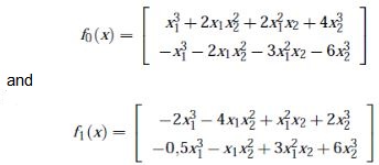
This system is considered to be a homogeneous switched system presented in stability analysis (Zhang et al., 2007). Polynomial equivalent representation is used to prove stability under arbitrary switching:

x^.(t)=f₀(1-s)+f₁s

s∈Γ ={s∈R/Q(s)=s(s-1)=0

Using these polynomial matrices and equation (27), the following is obtained:

-^δV/_δxf₀(1-s)+f₁(s)+(s⁴-2s³+s²)λ(x,s)≥0

Using SOSTOOLS, a Lyapunov function of degree six is found, i.e.

V(x)= -0,0364x²₁+0,02x⁴₁-0,0082x⁴₂+0,0476x²₂...

-0,056x₁x²+0,0113x²₁x²₂-0,064x₁x³₂-0,0457x⁶₁

...-0,016x⁴1x⁴₂+0,0034x⁶₂

which, through theorem 3.4, proves that the homogeneous nonlinear switched system reformulated as a polynomial DAE is stable.

Conclusions

This tutorial has presented SOS techniques as effective criteria for proving the non-negativity of multivariable polynomial functions. Although determining non-negativity of a function could be an NPhard problem, using SOS decomposition is an efficient method for solving this problem. Moreover, by means of the SOSTOOLS computational tool the problem can be simplified to (appropriately) use the SOS algorithm, taking into account the inherent numerical errors and high computational cost of this tool for relatively high order systems. Some SOS conditions are given for analysing rational systems with nonlinear controllers and switched systems using a polynomial approach based on stability analysis of nonlinear polynomial systems. The SOS techniques were used to consider the parameters' variations and possible uncertainties as inequality constraints on the original systems. Moreover, from the methods used to solve the presented examples it can be seen that SOS techniques are a useful method for dealing with high order and complex systems.