Efraín Domínguez¹, Felipe Ardila² y Santiago Bustamante³

¹ Hydrologist Engineer. M.Sc., in ecology Hydrometeorology. Ph.D., in technical sciences. Universidad Javeriana, Bogotá, Colombia.e.dominguez@javeriana.edu.co

² Systems Engineering, Universidad Distrital. M.Sc., student in Hydrosystems, Universidad Javeriana, Bogotá, Colombia. Geophysical Institute. felipeardilac@ gmail.com.

³Undergraduate, Universidad Javeriana, Bogotá, Colombia. santiagobus@gmail.com

ABSTRACT

Keywords: ODE solver, computational differentiation, modelling, dynamical system.

Received: june 23th 2009

Accepted: november 15th 2010

Introduction

Several real world problems can be studied using mathematical modelling methods. The differential operator is a widely-used operator for describing physical, biological, ecological and other types of processes. These processes are usually described through either an ODE of a different order r or a set of ODEs. Resolving these equations or sets of equations is often done by using numerical methods. For researchers interested in numerical solutions to their mathematical models, one has to be familiar with both numerical and programming techniques; however, this requirement delays research unless a specialist in numerical methods becomes available).

Automatic integration of ODE systems has been of interest for a long time. In fact, computational differentiation development (Tolsma and Barton, 1998) has been happening since the 1970s (Moore, 1979). Tolsma and Barton (1998) suggested five approaches to the computation of derivatives: hand-coding, finite-difference approximation, symbolic differentiation, evaluation using Reverse Polish Notation(RPN) (Bardsley and Prasad, 1997) and automatic differentiation. Iri (1991) described some prerequisites for a good differentiation method; it should be fast, free of truncation error and preferably performed automatically. Perhaps, however, an additional prerequisite should be considered. The method must allow generalisation to systems of any complexity. The second and fifth methods almost fulfil all of the mentioned requirements. Truncation errors are still present in the second method, however, and the fifth method requires high user intervention for providing a starting subroutine for calculating a given ODE system. Automatic differentiation could require some adaptation for solving problem sets in a discrete (tabular) manner. All of the above-mentioned techniques are used for solving modelling problems in different science domains and all of them are usually studied within the standard programme of a mathematical modelling course. There is a significant amount of specialised software on the market for solving ODE systems; most of this software is not available free of charge, however, and not all of the algorithms used are known as clearly as the researchers wish. The available applications do not provide the source code for the ODE system being investigated.

This paper presents the theoretical foundations, methods, algorithms and implementation of an automatic programmer and numerical solver for ODE Systems. This modelling system uses both Euler and Runge-Kutta explicit methods and export numerical solutions for visualisation within Scilab or Matlab packages. This application represents the first version of a modelling system implementing automatic code generation for solving differential equations when studying complex systems.

System Solver is open source software. It is a good tool for people who like to solve ODE although they are not programmers. This application is easier to use than programmes like Matlab because it only uses a few commands and it is specifically designed to solve ODE. System Solver is high-quality pedagogical software for an introduction to the world of mathematical modelling. The advantage of using System Solver instead of known programmes such as MatLab, Scilab or Octave is the teaching-orientated design aimed at developping modelling and programming skills at the same time. Another potential advantage is the possibility of choosing the language programme that users want to learn for modelled systems share code; such ability will be implemented in the next version of the package.

System Solver was developed in Java script and uses a special library named "Qt Jambi." It is an officially-supported technology aimed at all programmers who want to write rich GUI clients using Java language.

Compared to conceptual modelling tools like Stella, Powersim, Simile or Vensim, System Solver shows better explanatory power for basic modelling concepts. System Solver users can see the ODE behind the system they are simulating and they also have total control over a numerical code being used for solving the ODE system being studied. The design of n-dimensional problems in conceptual modelling systems can be troublesome because of the visual representation of the problem diagram. System Solver structure has been designed to allow a friendly setup of n-dimensional systems and the assimilation of partial differential equations to model distributed systems.

System-Solver structure

Using the following notation:

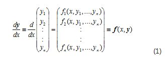
System (1) suggests a cyclical algorithm that applies a numerical method (Euler or Runge-Kutta in this case) ⁿ -times to find vector ^y (Боглаев, 1990). System Solver uses the Euler explicit finite differences scheme as follows:

It is also possible to select a fourth order Runge-Kutta explicit scheme in the form:

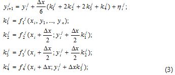
In both equations [(2) and (3)], n_i^j  represents an induced error due to the truncation of high order Taylor series derivatives during the deduction of finite differences for the ODE j . In fact,n_i→0 si Δx→0. Schemes (1) and (2) are both explicit and their performance depends heavily on the size of steps Δx. Index ⁱ fixes the ^x node that is being evaluated.

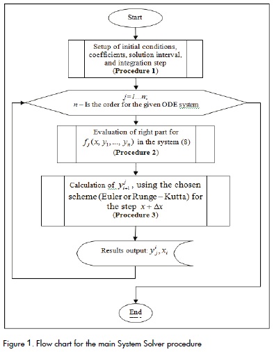
An experienced programmer will easily to recognise generic behaviour in equations (1), (2), and (3) for solving an ODE system. There must be a routine for evaluating y^j_i+1 (procedure 3 in Figure 1) and the right side of eq. (1) has to be solved using an external procedure (2 in Figure 1). The initial conditions, solution interval, ODE coefficients and integration step (Δx  ) must be setup. This can be done at the beginning of the calculations (procedure 1 in Figure 1). To solve the right side of functions, a parser procedure has been implemented leading to the identification of required variables and ODE parameters; ODE parameters can also be a function of time and/or the state variables of the system (1)

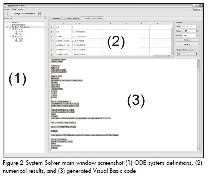
The basic System Solver structure is shown in Figure 2. This structure provides an interface for setting both the quantity of ODE in the studied system and also the fields for expressions defining right parts of the functions. A method called "Solve" activates the translation from algebraic notation to reverse Poland notation (RPN). The parameters, independent variables and state variables are classified from the RPN strings and used in previously-prepared code templates. The first template (RPEvaluator) evaluates the right parts of the expressions.

Once the RPEvaluator template is filled with the correct number of variables and the required ODE parameters, another template (EDOSystem) is completed with discretisation intervals, initial condition vectors and number of time steps. The EDOSystem is the implementation of the flow scheme presented in Figure 1. This procedure is the main procedure invoking a RPEvaluator instance that returns a solution vector for right parts of the equation required by the Runge- Kutta or Euler procedures and creates a new evaluation y^j_i+1  for every time node ^x .

Some dynamic systems are examined and their hand-code and System Solver solutions compared as an example. Consider a predator-prey system of the type:

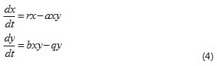
Here, ^r and ^q are growth coefficients and ^a and ^b are the predator's attack rate and its reproductive efficiency, respectively.

Given initial conditions,

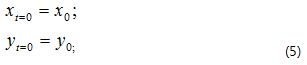
An experienced modeller would find the numerical solution of (4) using the Euler methods.

Following the structure shown in Figure 1, the ODE_Euler system is equivalent to Procedure 1 in Figure 1, the sub right(.) is the equivalent of Procedure 2, and the sub Euler(.) evaluates x_t+1  and   y_t+1  y (procedure 3 in Figure 1).

The ODE system must be set up to solve the same problem within the System Solver application by adding each equation at once using the common notation used in spreadsheet applications to define mathematical expressions. The order of the ODE system is only restricted by the hardware specifications. Figure 2 describes the main System Solver window. This application is user-friendly, even for scientists having minimal knowledge of modelling, numerical methods, and programming. A model setup requires no more than a couple of minutes to complete. The researcher expends time in finding the required equations, defining the numerical values of parameters and interpreting results instead of designing, coding and debugging a numerical algorithm.

For the case of the predator-prey model (Equation 4), System Solver provides the Visual Basic code shown in http://www.mathmodelling.org/home/System Solver-1

The System Solver Visual Basic code can be pasted directly to a Microsoft Excel Visual Basic module. It can then be used as a Macro to obtain model results placed directly into a sheet in the current Workbook. The generated code can also be prepared for the MS Visual Basic stand alone compiler. This compiler can be downloaded from the Microsoft web site: http://www.microsoft.com. The open source "Mono" project sponsored by Novell has included a Visual Basic compiler in its integrated development environment. This compiler allows MS Visual Basic code to run in different operating systems, including Linux, Mac OS X, Sun Solaris, BSD - OpenBSD, FreeBSD, NetBSD and Microsoft Windows. More information about the "Mono" project can be obtained from: http://www.monoproject.com.

If the System Solver code is generated for a stand-alone Visual Basic compiler, it is necessary to edit the output code to permit post-processing. Independently of the platform for which the code is generated, the Scilab or Matlab packages offer one post-processing option. System Solver can save numerical results to an ASCII formatted text file and generate the required script to provide rapid graphic output in Scilab or Matlab environments.

Solving a third order ODE system and exporting the results to the Scilab and Matlab packages

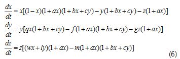
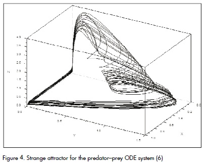
Many modelling problems include three or more ODEs in the system to describe a phenomenon being studied. Such multidimensional systems require 3D graphic abilities during post-processing. In the System Solver case, such abilities are provided by the export option which prepares the results to be processed with the Scilab or Matlab packages. The discrete solution is exported to a text file and an import script that imports the resulting data to the selected package (Scilab or Matlab) is provided. A three-dimensional competition model given by the system can be solved to examine this ability (Saez et al., 2007):

with initial conditions:

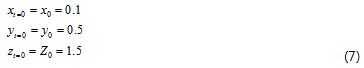
using the following parameters: a=1.5, b=5.0, c=8.0,q=1.0, f=0.16, g=0.1, w=1.1 , l=2.0, m=0.16, Δt=0.1, t_min=0, and. Entering this setup into System Solver provides us with the Visual Basic code listed in Figure 2.

The Solver System "export" function saves the resulting data and a Scilab script within a user-selected location. The script is presented in Figure 3.

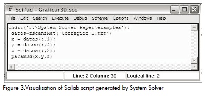
Loading and executing the Script in the Scilab environment produces the graphing shown in Figure 4.

Conclusions

The examples presented show that the System Solver prototype is able to handle ODE and PDE problems of differing complexities. This version can write efficient numerical code and provides tools for exporting the numerical results to Scilab and Matlab programmes enabling 3D graphical presentation of problem output. The application presented here offers a helpful tool for modelling systems represented by sets of ODEs. All of these abilities accelerate research when dealing with ODE systems and they also support teaching efforts in programming, mathematical modelling and numerical methods courses. Using System Solver closes the cycle of defining a mathematical model, building a numerical algorithm and coding a programmeto simulate a dynamic system (Samarsky and Mikhailov, 1997).

System Solver's ability to switch between the Euler and fourth order Runge-Kutta methods allows exploring their properties for each ODE system investigated.

System Solver has been thought to act as a cross platform system. It is projected that future System Solver versions will provide source code for several compilers, such as C#, C++, Java, object-oriented Pascal, component Pascal and Fortran compilers. At the moment,output source code is written for Visual Basic compilers and Visual Basic for applications interpreters (like the one included in MS Office applications). A Visual Basic compiler is also available for the Mono project so the produced code can also be executed in Linux and other UNIX-like systems. A beta version of System Solver can be downloaded from the website: http://www.mathmodelling.org/home/System Solver-1

It is envisioned that several numerical algorithms for solving ODE systems, including algorithms for stiff (rigid) equations, will be provided by System Solver in the near future; algorithms for solving stochastic differential equations will also be implemented. Suggestions regarding user requirements from System Solver users are welcome.