Elkin Florez¹, Yamid Carranza², Yesid Ortiz³

¹Mechanical Engineer, Universidad Francisco de Paula Santander, Colombia. Master of Mechanical Engineering, Universidad de los Andes, Colombia. Master in Chemical and Process Engineering, Universidad de Rovira i Virgili, Spain. Doctor in Mechanical Engineering, Aeronautics and Fluid, Universidad Politécnica de Cataluña, Spain. Associate Professor, Universidad de Pamplona. eflorez@unipamplona.edu.co

² Mechanical Engineer, Universidad Tecnológica de Pereira, Colombia. Master of Mechanical Engineering, Universidad de los Andes, Colombia. PhD Student, Politécnico de Monterrey, México. Assistant Professor, Universidad Tecnológica de Pereira, Colombia. yamidc@utp.edu.co

³ Mechanical Engineer, Universidad Francisco de Paula Santander, Colombia. Master of Mechanical Engineering, Universidad de los Andes, Colombia. Assistant Professor, Universidad Tecnológica de Pereira, Colombia. yosanchez@utp.edu.co

ABSTRACT

Numerical solutions of 2-D laminar flow over a backwardfacing step using the lattice Boltzmann equation method (LBEM) are presented in this article. Unlike conventional numerical schemes based on macroscopic continuum equation (mass conservation and Navier-Stokes) discretisation, the LBEM is based on microscopic models and mesoscopic kinetic equations. The simulations were validated for a wide range of Reynolds numbers (100 ≤ Re ≤ 1,000), comparing them to previous studies. Several flow features, such as primary and secondary vortex location at the bottom and top of the wall, respectively, were investigated regarding Reynolds number. Two typical classes of boundary condition were implemented in the LBEM model: the Drichlet condition at the inlet flow (parabolic speed profile) and the Newman condition at the outlet flow (zero gradient speed). The results showed that the LBEM gave accurate results over a wide range of Reynolds number; these were compared with other numerical methods and experimental data.

Keywords: fluid flow, lattice Boltzmann equation method, numerical simulation.

Received: February 16th 2010

Accepted: May 25th 2011

Introduction

Flows through channels where there is separation and recirculation of the boundary layer is often found in many flow problems in engineering. Typical examples would be flows in a heat exchanger and pipelines. A backward-facing step (BFS) flow can be considered to be the simplest geometry having great physical content shown by the vortices that are presented and their recirculation, all of these depending on the Reynolds number (Re) and the aspect ratio parameter.

In the literature one can find many numerical studies of a twodimensional, incompressible and stable BFS flow. Controversy can be identified in these studies regarding whether a stable solution for Re > 800 can be obtained. This has been discussed in detail by Gresho (Gresho et al., 1993) who concluded that the BFSF is stable and computable at Re = 800. Other authors (Keskar and Lyn, 1999; Barton, 1997; Sheu and Tsai, 1999; Biagioli, 1998; Erturk, 2008) have presented BFS flow solutions above Re = 800, using different methods for the discretisation of traditional Navier-Stokes equations.

LBEM has been the object of high paced development and has become a powerful method for simulating fluid flows (Moahamad and Kuzmin, 2010). However, many issues need more investigation and critical evaluation. The method has also been used by some authors paying less attention to LBEM parameter limitations and constrains. Some of these issues concern the treatment of boundary conditions, initial conditions and relaxation time, these being the topics being studied in the present paper.

The LBEM is an explicit time finite difference scheme for continuous Boltzmann equation in phase space and time (He and Luo, 1997). The LBEM has a underlying Cartesian lattice grid in space as a consequence of discrete speed set symmetry and the fact that lattice spacing Dx is related to time step size Dt by Dx = cDt, where c is the basic discrete speed set unit. This makes the LBEM a very simple scheme as it consists of two essential steps: collision and advection. Collision models various interactions amongst fluid particles and advection simply moves particles from one grid point to another, according to their speed. LBEM simplicity and kinetic nature are among its appealing features.

LBEM are based on the original idea of lattice gas cellular automaton (Frisch, 1986). A mesoscopic scheme is used to simulate fluid motion within the lattice, where time step is unitary and there is discrete phase-space. Each cell represents an element of fluid volume in the domain grid; the volume element consists of a group of particles whose motion is specified by a particle distribution function (pdf). In the classical model, the pdf is the Maxwell-Bolztamnn distribution. The particles move to adjacent cells, according to the model selected at each time step (propagation step) and collide with other particles coming from or traveling to the same cell in different directions (step collision). Macroscopic variables such as density and speed are calculated from the pdf (Maxwell, 1997) (Dieter, 2000).

The backward facing step flow has been numerically solved for a wide range of Reynolds numbers 100 ≤ Re ≤ 1,000 in this work to determine LBEM effectiveness and the method' s accuracy has been determined, comparing and making a brief discussion of data regarding both numerical and experimental results obtained by other authors.

Solution method

The LBEM' s guiding principle is to construct a dynamic system on a simple high-symmetry lattice (mostly square in 2D and cubic in 3D) involving a number of quantities which can be interpreted as the pdf of fictitious particles on the lattice links. These quantities then evolve in discrete time according to certain rules chosen to attain some desirable macroscopic behavior emerging on large scales relative to lattice spacing (Lalleman and Luo, 2000). The lattice Boltzmann equation has been defined (He and Luo, 1997; Dieter, 2000; Succi, 2001) as:

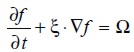[1]

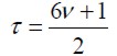
where Ω is the collision operator. This term can be simplified significantly using the Bhatnagar-Gross-Krook approximation (BGK), using a single relaxation time t (SRT) which is the simplest method used for solving the equation (1). This involves replacing the collision term by a term that relates the difference between function f and the Maxwell-Boltzmann equilibrium function with determined relaxation time.

The basic premise for using these types of simplified kinetic methods for macroscopic fluid flows is that the macroscopic dynamics of a fluid result from the collective behaviour of many microscopic particles in the system and that macroscopic dynamics are not sensitive to underlying details in microscopic physics. By developing a simplified version of complicated kinetic equations, such as the full Boltzmann equation one does not have to follow each particle, as in molecular dynamics simulations (Chen and Doolen, 1998). The LBEM can be written as:

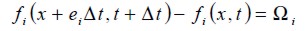[2]

where f_i(x,∪,t), are the particle distribution function, x and υ being position and particle speed, respectively, in phase space (x, υ) and time t. Here macroscopic quantities such as speed and density can be obtained through the first moments of f (x,υ,t). Collision operator Ω, on the right-hand side of equation (2) using the BGK approximation, will be replaced by (Dieter, 2000):

where fi^(eq)(x,t) is the equilibrium distribution function, e_i are discrete speed vectors and τ is relaxation time related to fluid kinetic viscosity (He and Luo, 1997):

[3]

[4]

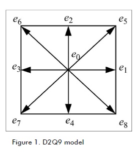
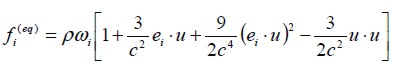
Figure 1 shows the standard D2Q9 lattice model (two-dimensional and nine discrete speeds) used in this work where equilibrium distribution function is defined by isothermal and incompressible flows as (Quian, 1992):

[5]

where ρ and u are macroscopic speed and density, respectively, and ω_i constant weight factor, for D2Q9 given as:

[6]

Discrete speeds, e_i, for D2Q9 (Figure figura 1) are defined as follows:

where c=Δx/Δt=Δ and /Δt, Δx y Δt are lattice space and lattice time step size, respectively, being set to unity. The basic hydrodynamic quantities are obtained through moment summations in the speed space

[7]

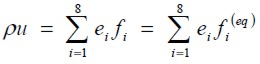[8]

Macroscopic viscosity is determined by

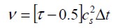[9]

where c_s is the speed of sound and equal to c/Ö-3 (Mohamad et al., 2010).

The evolution of the medium, for the BGK model, consists of two steps: streaming (motion towards relevant neighbours) and collision (redistribution of the f' s at each node). These are calculated by means of:

Collision step:

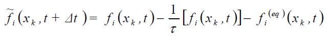[10]

Streaming step:

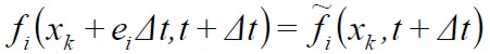whereƒⁱ, represents the post-collision step. The post-collision step is totally local and the streaming step does not require large computational effort (Quian, 1992) (Maxwell, 1997).

Backward-facing step model

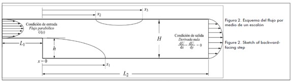
Figure 2 shows the scheme for the flow considered in the current study. Here, flow entry was located up-stream from the step and was placed at L₁ = 4h behind the step and the exit was located L₂ = 35h down-stream of the step. The number of horizontal nodes was N_x = (L₁ + L₂). Channel length to the exit was selected bearing in mind that flow recirculation points were not affected by the same exit condition. Channel height was defined as H = 2h.= N_y-2, where Ny was the number of nodes in the channel' s vertical direction. The lattice was completely uniform in the whole domain. Distance x₁ determined the point where flow recirculation appeared near the bottom of the channel' s low and distances x₂ and x₃ defined recirculation points at the top of the wall. All distances were indexed to the step, in x = 0, according to t Figure 2.

Inlet flow condition

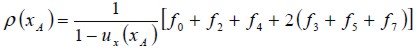
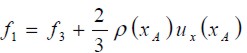
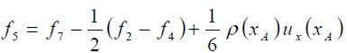
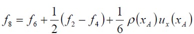
Barton (1997) studied the effect of channel length on flow upstream of the step (inlet flow) and demonstrated that the numerical flow solutions so obtained were only affected for low Reynolds numbers. In this research, this length was selected as being equal to L₁ = 4h. The assumption was that flow was completely developed (like Poiseuille flow) between two flat plates, equivalent to imposing a parabolic profile for speed (U = u_x, u_y = 0). Unknown distribution functions for nodes at the inlet were calculated using the f ^{' s} derived from those within the domain and their corresponding speed value. For the D2Q9 model, and taking node xA as an example (shown in Figure 3), f₀, f₂, f₃, f₄, f₆, and f₇ became known after the propagation step because they were derived from nodes neighbouring x_A, and functions f₁, f₅, and f₈ were calculated using equations (7) and (8), as was equality for the non-equilibrium distribution function in a normal direction at the inlet flow. These were determined as follows:

[11]

[12]

[13]

[14]

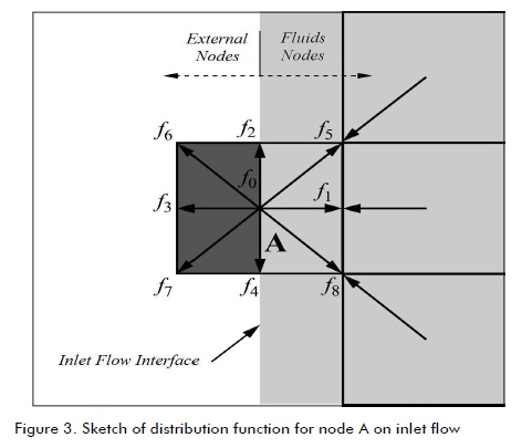
Taking equation 10 into account in the collision step, then had to be obtained for i = 1, 5 and 8. Calculating the unknown f ^{' s} needed special treatment to avoid the loss of particles in both the top and low corners.

Outlet flow condition

Here, two types of conditions were verified. A fixed speed flow (i.e. Drichlet condition) was first implemented at inlet and outlet flow imposing a parabolic speed profile, the difference being that the f^{' s} to be calculated at the outlet were f₃, f₆, and f₇. The null derivative condition for outlet flow speed was also studied (Newman condition) where the value of speed in the exit node had the same value as the immediately previous node in direction x. These conditions have been seen to not greatly affect flow (Zou y He, 1997; Bouzide, et al., 2001; Latt, 2008).

Fixed boundary condition

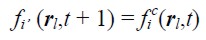
The linear approach, proposed by Bouzidi (2001), known as bounce-back, was used to treat the propagation step in the presence of a fixed wall where the wall was located halfway between the solid and fluid nodes. Supposing that rl described fluid node position f, then r_l + e_i would be solid node position and assuming e_i' were inverted speed or inverse direction for e_i, namely (e_{i '} = -e_i), then:

[15]

On the right-hand side of the equation ((15)), f ^c was taken after collision and before propagation. f ( ,t + 1) would then be used for values after collision and propagation, corresponding to a completed LBM time step. The previous factor indicated that solid and fluid node dynamics, wall neighbours, only differed regarding the propagation step (Flórez, 2008).

Results and Discussion

The computational code for developing the flow diagram was proposed by Flórez (2008); Fortran 90 programming language was used. Latt (2008) was used for defining/selecting LBM unit values, bearing existing theory in mind and the method' s limitations, these being t = 0.54 relaxation time, U_max = 0.057 maximum speed at inlet channel, Re = 2h-·_max/3n Reynolds number where n was obtained from equation 9, N_x the number of nodes used and N_y a function of Re to be simulated. The respective values were: Re = 100 N_x = 850, N_y = 52, Re = 200 N_x = 1.700, N_y = 102, Re = 300 N_x = 2.550, N_y = 152, Re = 400 N_x = 2.550, N_y = 152 y, para Re > 500 N_x = 4.250, N_y = 252.

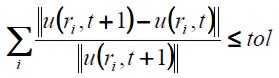
Equation (16) shows where r defined a node' s coordinates and t the time. The speed calculated throughout the whole domain was the criterion of convergence used in all simulations. Looking for high accuracy in the results, tolerance was defined by, tol = 10^-7.

[16]

Figure 4 shows speed fields and their respective flow streamlines for 100 ≤ Re ≤ 1,000. The speed fields show how speed magnitude became distributed inside the channel as the number of Re increased. The streamlines allowed observing vortex formation. It can be noticed that in this Figure the scale in x and y direction have been manipulated to clearly identify difference regarding the different details present in the flow for the whole rank of Re numbers. Moreover, it should be stressed that the streamlines allow clearer observation of the appearance of recirculation at the top of the wall for Re ³ 400. The results for the whole range of numbers for Re100 ≤ Re ≤ 1,000 have been compared to numerically and experimentally ones obtained by other authors; in most cases this flow has been investigated up to Re = 800.

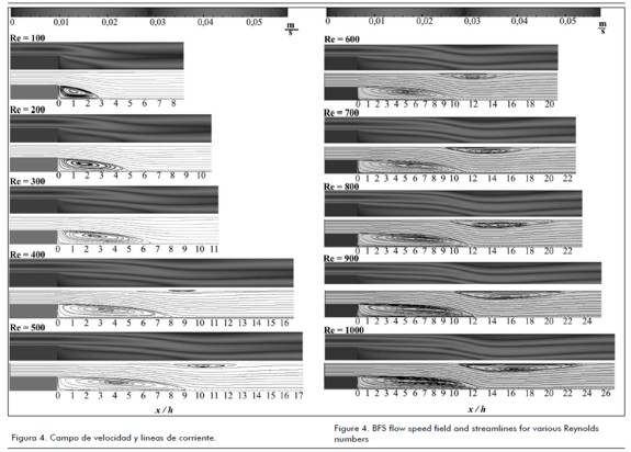
Figure 5 shows the position of the first recirculation point or vortex present at the channel' s low wall compared to computational results obtained by Kanna et al., (2006) and Erturk (2008) and experimental results obtained by Armaly et al. (1983).

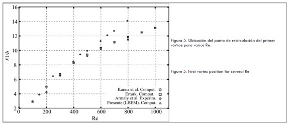
Figure 6 shows recirculation points or vortex generated at the channel' s top wall. This was compared (Figure 5) to other authors' numerical and experimental results.

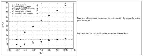
Table 1 shows the numerical results obtained for recirculation point coordinates using the LBEM.

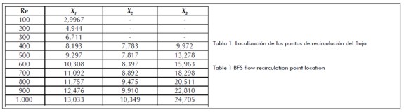
Recirculation point coordinates were calculated for the whole of the x direction. Fluid node speed was taken immediately after the low wall (y = 2) to determine coordinate x1 for the first recirculation and immediately prior to vertical fluid node at the top of the wall (y = Ny-1) to determine second recirculation coordinates x₂ and x₃.

Conclusions

The steady state backward-facing step stable state problem has been numerically resolved using the lattice Boltzmann equation method. A parabolic speed profile was used at inlet flow and the null derivative condition at the outlet in such simulation. The outlet flow was located downstream from the step sufficiently away from it so that the vortex generated in the flow was not affected by the outlet. Different mesh sizes were used, from 850 x 52 for Re = 100, up to 4250 x 252 for Re = 1,000. The lattice Boltzman method has been seen to give highly accurate numerical results for simulating laminar flows in the presence of a vortex An important point was revealed in the recirculation generated by the flow at the top of the wall. This recirculation reflected a single-vortex pattern for all Re numbers, unlike the simulation for Re = 800 where three vortexes were revealed in the same recirculation (See Figure 4). The authors believe that the pattern mentioned above was due to Re = 800 being a flow transition point and that flow was not completely stable from this Re onwards.

References

Armaly, B. F., Durst, F., Pereira, J. C. F., Schonung, B., Experimental and theoretical investigation of backward-facing step flow., Journal of Fluid Mechanics, 127, 1983, pp. 473-96. [ Links ]
Barton, I. E., The entrance effect of laminar flow over a backward -facing step geometry., Int J. Numer. Methods Fluids, 25, 1997, pp. 633-44. [ Links ]
Biagioli, F., Calculation of laminar flows with second-order schemes and collocated variable arrangement., Int J. Numer. Methods Fluids, 26, 1998, pp. 887-905. [ Links ]
Bouzidi, M., dÂ'Humieres, D., Lallemand, P., Luo, L., Lattice Boltzmann Equation on a Two-Dimensional Rectangular Grid., Journal of Computational Physics, 172, 2001, pp. 704-717. [ Links ]
Dieter, A. Wolf-Gladrow., Lattice-Gas Cellular Automata and Lattice Boltzmann Models, Springer (ed.), 2000, pp. 40-65 [ Links ]
Erturk, E., Numerical solution of 2D steady imcompressible flow over a backward-facing step, Part I: High Reynolds number solutions., Computer & fluids, 37, 2008, pp. 633-55. [ Links ]
Florez, S. E., Cuesta, I., Salueña, C., Flujo de Poiseuille y la cavidad con pared movil calculado usando el método de la ecuación de lattice Boltzmann., Ingeniería & Desarrollo, 24, 2008, pp. 117-32. [ Links ]
Frisch, U., Hasslacher, B., Pomeau, Y., Lattice-gas automata for the Navier-Stokes equation., Phys. Rev. Lett, 56, 1986, pp.1505-1515. [ Links ]
Gresho, P.M., Gartling, D.K., Torczynski, J.R., Cliffe, K.A., Winters K.H., Garratt T.J., Is the steady viscous incompressible two-dimensional flor over a backward-facing step at Re =800 stable?., Int J. Numer., Methods Fluids, 17, 1993, pp. 501-41. [ Links ]
He, X., Luo, L-S., Theory of the lattice Boltzmann method: From the Boltzmann equation to the lattice Boltzmann equation., Phys. Rev. E, 56 (6), 1997, pp. 6811-17. [ Links ]
Kanna, P. R., Das, M. K., A short note on the reattachment length for BFS problem., Int J. Numer. Methods Fluids, 50, 2006, pp. 683-692. [ Links ]
Keskar, J., Lyn, D.A., Computation of laminar backward-facing step flow at Re = 800 with spectral domain decomposition method., Int. J. Numer, Methods Fluids, 29, 1999, pp. 411- 427. [ Links ]
Latt, J., Choice of units in lattice Boltzamnn Simulation., Lattice Boltzmann Howtos: http://www.lbmethod.org/howtos:main. 2008. [ Links ]
Maxwell, B. J., Lattice Boltzmann methods in Interfacial Wave Modelling., Ph. D. Tesis. Edinburgh's University, 1997. [ Links ]
Quian, Y., d'Humieres, D., Lallemand, P., Lattice BGK models for Navier-Stokes Equation., Europhys. Lett., 17, 1992, pp.479-84. [ Links ]
Sheu, T., Tsai, S., Consistent Petrov Galerkin finite element simulation of channel flows., Int J. Numer. Methods Fluids: 31,1999, pp. 1297-310. [ Links ]
Succi, S., The lattice Boltzmann Equation for Fluid Dynamics and Beyond. Oxford (ed.), 2001, pp. 64- 93. [ Links ]
Zou, Q., He, X., On pressure and velocity boundary conditions for the lattice Boltzmann BGK model. Phys Fluids: 9, 1997, pp. 1591-1598. [ Links ]
All the contents of this journal, except where otherwise noted, is licensed under a Creative Commons Attribution License
Tel-fax (57 1) 3165000 Ext. 13374
revii_bog@unal.edu.co