Recommendations for grounding systems in lightning protection systems

Recomendaciones para el diseño de la puesta a tierra en los sistemas de protección contra rayos

Johny Montaña²

¹ Electrical Engineer, M.Sc. in High Voltage and Ph.D. in Electrical Engineering from National University of Colombia. He is a Professor of Universidad del Norte and is with the Power System Research Group-GISEL, Barranquilla - Colombia, e-mail: johnym@uninorte.edu.co

ABSTRACT

Keywords: method of moments, hybrid electromagnetic method, grounding configuration, grounding impedance, transient voltage

RESUMEN

Palabras claves: método de momentos, método electromagnético híbrido, configuraciones de puesta a tierra, impedancia de puesta a tierra, tensión transitoria.

1. Introducción

AN integral lightning protection system consists of three elements: external protection systems (air terminations, down conductors, earth terminations), an internal protection system and personal safety guide. Risk assessment is carried out according to IEC 62305 for establishing the need for a lightning protection system in a particular facility. Risk assessment takes aspects such as building materials, height, volume, purpose and the area's lightning density into consideration.

If an external protection system is required, the rolling sphere method (IEEE Std-62305) can be used for determining the location of air terminations and down conductors. The earth terminations can be defined by means of an International Electrotechnical Commission (IEC) standard table, taking soil resistivity and protection level into account and giving the electrodes' length or by means of specialised software.

Some technical books, standards and papers present typical configurations regarding earth electrodes for buildings, towers, poles, houses, etc (IEEE Std-62305; Casas, 2008). Some of these configurations can be modified for obtaining better results concerning transient phenomenon. This paper presents a transient analysis of some such configurations to ascertain how they can be modified to get better earth electrode results.

The results presented in this papers were obtained by means of specialised software developed using the hybrid electromagnetic method (Montaña, 2006a; Montaña, et al 2006b). Impedance and voltage results are shown to provide recommendations for geometry, injection point location, rod electrode location, mesh size, etc.

2. Hybrid Electromagnetic Method (HEM)

A methodology was used for describing structures' electromagnetic behaviour, which may be represented by cylindrical conductors (Montaña, 2006a; Visacro, 1992a; Valencia, Moreno, 2003; Visacro, 1992b). Grounding system conductors are partitioned into a number of segments, according to method of moments (MoM) (PCB-MoM) using thin wire approximation. Each is considered to be an electromagnetic field source produced by a transversal current (It) and a longitudinal current (Il) which are constant throughout each segment (Figure 1).

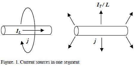
The electromagnetic coupling between each pair of segments is calculated by using the expressions for scalar and magnetic vector potentials and assuming an average potential V for segment and a voltage drop AV on it. Coupling impedance matrices Zt and Zl are thus calculated.

Once this has been done, circuit relationships between voltages and currents allow the system to be represented in a compact form and solved for its nodal voltages (unknown). Once these voltages have become known, the current distribution throughout the grounding system can also be ascertained.

Since all the calculations involved in this methodology are carried out in the frequency domain, soil parameters, skin effect and propagation effects' frequency dependence are easily included. Such methodology is used in this paper to find earth electrodes' input impedance frequency response by means of the voltage-current relationship. Responses in the time domain are computed by means of the inverse Fourier transform (IFT) (Montaña, 2006a) from the responses in the frequency domain.

3. Parameters analysis

Impedance in the frequency domain and voltage in the time domain were computed using the HEM-based software to compare different arrangements. The impedance analysis was performed from 100 Hz up to 3 MHz, due to most representative lightning phenomenon components occurring within that range.

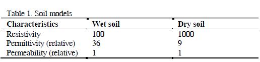
Soil was modelled by means of permittivity, permeability and resistivity values. Two soil models were used to carry out the simulation (Table 1) (Grcev, 1993).

A. Triangle or wye configurations

The first configurations being studied were triangle and wye configurations; they were named according to the geometric figure formed by their conductors (Figure 1).

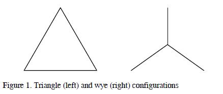
Figure 1. Triangle (left) and wye (right) configurations

These configurations are used in simple lightning protection systems where it is not possible to use counterpoises or mesh grids. The down conductor is connected in one corner for triangle configuration or is connected at the centre point for wye configurations. Figure 2 shows the impedance values at the injection point for both configurations. Simulations were made for both soils defined in Table I. Each conductor was 5 m in length, 0.5m depth and had 0.01 m radii.

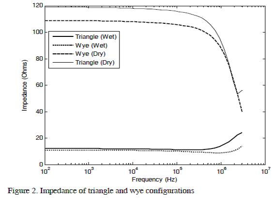
This simulation was used for defining which of the two configurations presented the lower impedance values at the injection point. The results showed that the wye configuration presented the lower impedance values for wet or dry soil. Taking into account that both configurations used the same conductor length, it was better to build the second one (wye configuration).

B. Counterpoise effective length

A simulation was developed to define the maximum length of counterpoises to be used in grounding systems; a 100 m, 0.01 m radii counterpoise, buried 0.5 m, was modelled. The simulations were developed in both soil types at 100 Hz and 2 MHz frequency. The injection point was at the beginning of the counterpoise. Figure 3 shows current distribution per unit throughout the counterpoise.

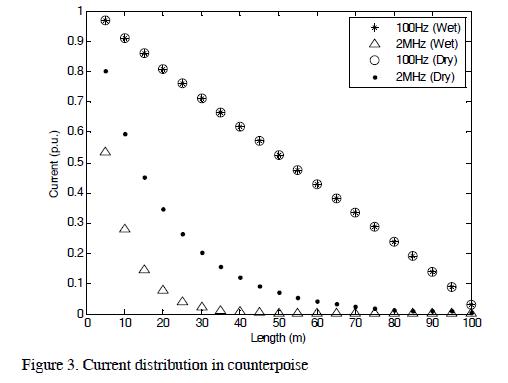
Figure 3 shows current variation throughout the counterpoise for two types of soil. Distribution was uniform at low frequency and had no dependence on soil type; however, distribution was highly dependent at high frequency. The current was scattered during the first meters (around 40m) for wet soil while current was almost zero for lengths greater than 70m for dry soil. That meant that transient analysis showed that using greater than 70 m counterpoise length was a waste of money because the current was going to be scattered during the first meters nearest to the injection point. Furthermore, the inductive effect in very long counterpoises could increase impedance magnitude. On the other hand, there is not limit to counterpoise length in AC analysis because the current is uniformly distributed. However, grounding electrodes are used nowadays in AC and transient at the same time so maximum counterpoise length should be close to 70 m in high resistivity soils and 40 m in low resistivity soils.

C. Counterpoise with or without rods

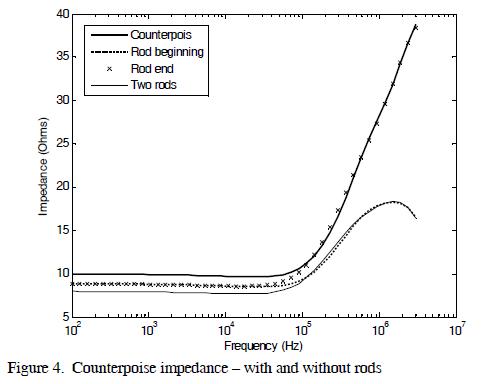
The impedance magnitude values of a counterpoise with and without rods is presented. The rods were located at the beginning and in the open end. The counterpoises were modelled with 0.01m radii, 15 m length and buried 0.6 m; the rods measured 2.4 m in length and had 0.01 m radii. They were modelled in wet soil.

Figure 4 shows the difference between impedance at the injection point when the rods were not included, when the rod was included at the beginning, at the open end and at both the beginning and open ends. The results showed that better performance was achieved when the rod was included at the beginning of counterpoise, because including the rod at the open end led to no significant differences at high frequencies.

D. Counterpoises length

The impedance magnitude values for different length counterpoises was presented. The cables were modelled having 0.01m radii and buried 0.6 m in wet soil.

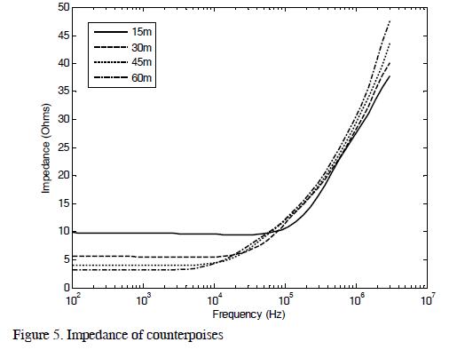
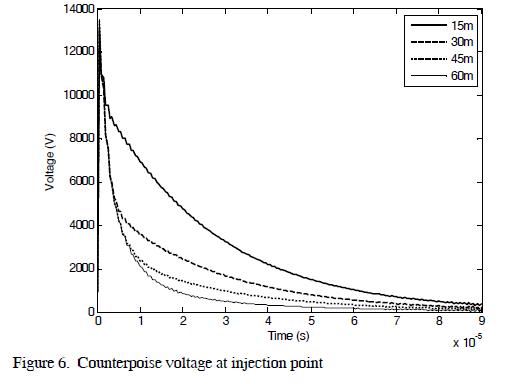
The counterpoise impedance values had no important variations regarding counterpoise length at high frequencies, meaning that the transient response of different counterpoise lengths was the same. The voltage of four counterpoises was modelled in the time domain to complement this analysis; current was 1 kA and 1/20 ms. The results are shown in Figure 6.

Figure 6 shows injection point voltage for each counterpoise. The peak values for four counterpoises were the same; the differences shown in the tails of the waveforms explained because impedance magnitude had variations at low frequencies but not at high frequencies. It may thus be concluded that increased counterpoise length modified transient voltage tail but not the peak.

E. Voltage throughout the counterpoise

Transient voltage is presented at three different points on a counterpoise measuring 60 m length, 0.01 m radii, buried 0.5 m. The simulation was carried out with wet soil parameters in the time domain when the current was 1 kA and 1/20 ms. Figure 7 shows transient voltage at the injection point, centre point and open end of the counterpoise.

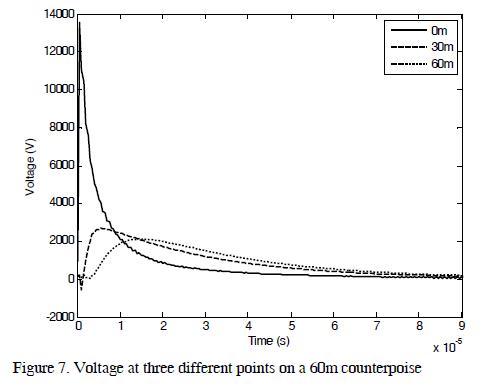
Based on these results, it is shown that the concept of ''equipotentiality'' has a different meaning in transient analysis, since (as shown in Figure 7) there was a voltage difference between points on the same conductor and the peaks happened at different times. It would thus be advisable to connect different devices at the same grounding system point to avoid large voltage differences which could damage a device's insulation.

F. Mesh for different areas

Different sized meshes' impedance values are now presented. The meshes were modelled in wet soil, built with a 0.01 m radii conductor, buried 0.5 m. The meshes were defined by means of the number of inner grids; the distance between conductors in both directions was 6 m (constant). For example, 1x1 mesh had one grid (6x6 m), 4x4 had sixteen grids (24x24 m) and 8x8 had sixty-four grids (48x48 m). All meshes were injected at one corner. Figure 8 shows the results.

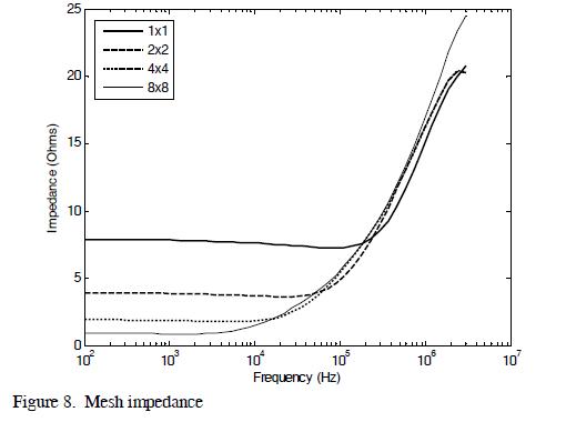
From Figure 8, it was concluded that the high frequency impedance value had no large variation for the four different meshes being studied; variation took place at low and medium frequency (up to 100 kHz), meaning that differences were again presented in the time domain in the tail of the transient voltage.

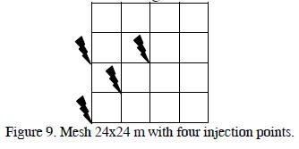
G. Injection point dependence in a mesh (impedance)

Impedance was simulated at four injection points in a 24x24 m mesh having 16 inner grids to determine injection point dependence in the impedance value (see Figure 9). The mesh was modelled in wet soil, built with conductors measuring 0.01 m radii, buried 0.5 m. The impedance for four injection points are shown in Figure 10.

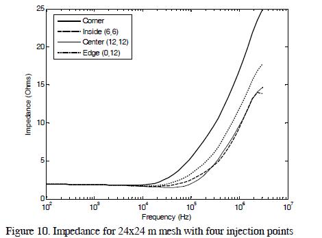
Injection point dependence is presented in Figure 10. The differences were noticeable at frequencies over 10 kHz, becoming lower when the injection point was located in the centre of the mesh and higher at the corners. The differences were thus shown at peak transient voltage not in the tail, as will be shown in the next section. Notice that the same mesh may depict diverse performance depending on the injection point.

H. Injection point dependence in a mesh (voltage)

To support the above conclusion, the same mesh was fed with 1 kA and 1/20 m current . The current was injected at the centre point and in the corner (Figure 11).

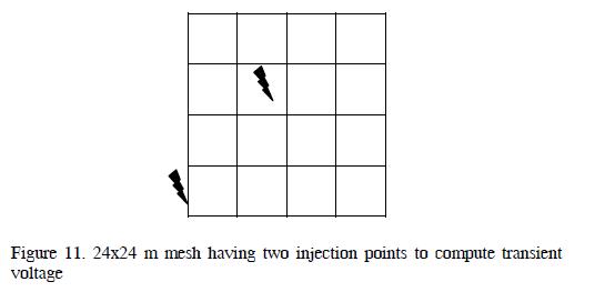
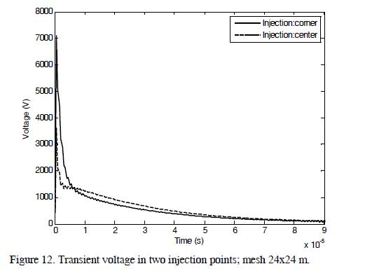
Figure 12 shows the differences between transient voltage when the injection point was in the centre and in a corner. The differences mainly occurred in peak waveform not in the tail; the differences were almost twice higher when the injection point was located in a corner.

I. Voltage difference in a mesh

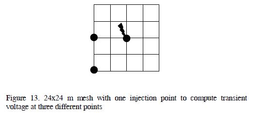
Continuing mesh analysis, voltages were then found at different points in the same mesh (24x24m) when current was fed at the centre point to identify voltage difference in the same system due to transient performance. The transient voltage was computed at the injection point (centre), in a corner and at the edge of the mesh (Figure 13).

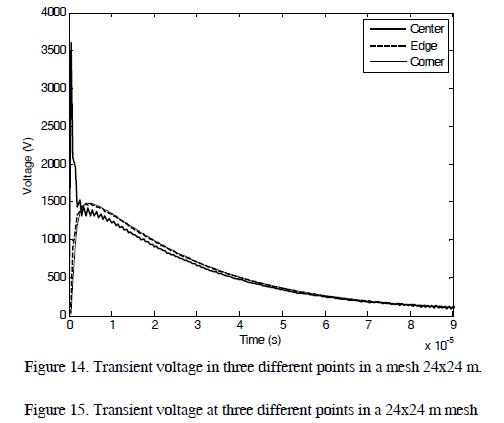
As was concluded in Figure 7, when a grounding electrode was analysed in the transient domain, it had voltage differences between points within itself. Figure 14 shows that the differences were obvious when the observation point was moved. In this case, the difference between the centre point and the corner was 1.5 kV when the transient voltage in the injection point was 3 kV peak.

4. Conclusions

Based on the transient analysis of grounding configurations it may be concluded that:

• When there is not enough area to build grounding electrodes, it is better to use a wye configuration instead of the triangle configuration;
• Effective counterpoise length was close to 70 m in high resistivity soils and 40 m in low resistivity soils;
• The best performance was achieved when a rod was included at the beginning of a counterpoise, not at the open end;
• Increasing counterpoise length modified transient voltage tail, not its peak;
• The down conductors had to be connected in the centre of the meshes, not in the corner or at the edges, to reduce impedance; and
• When a grounding electrode was analyzed in the transient domain, it had voltage differences between its points so that it should be mandatory to connect different devices at the same grounding system point to avoid large voltage differences.

5. Ackowledgment

The author wishes to express his gratitude to COLCIENCIAS and Universidad del Norte for financing this work.

6. References

Casas, F. (ed), Tierras, soporte de la Seguridad Eléctrica, 4a ed., 2008.        [ Links ]

Grcev, L., More Accurate Modeling of Earthing Systems Transient Behavior, 15th Telecommunication Energy Conference, INTELEC, vol. 2, pp. 167-173, 1993.        [ Links ]

IEEE Std. 62305, Protection against Lightning Part I, II, III.        [ Links ]

Montaña, J., Grounding system, Soil electric parameters variation with frequency and software for computing transient voltages, Thesys, National University of Colombia, Doctor of Philosophy, 2006a.        [ Links ]

Montaña, J., Montanyá J., et al, Quasi-static approximation of concentrated ground electrodes: experimental results, 28th International Conference on lightning protection, ICLP, Kanasawa - Japan, 2006b.        [ Links ]

PCB-MoM Software Manuals, A method of Moment Program for Radiated Emission and Susceptibility Analysis of Printed Circuit Board.        [ Links ]

Valencia, J., Moreno, G., Modelación de puestas a ierra para evolución de sobretensiones transitorias, Congreso Iberoamericano de Alta Tensión y Asilamiento Eléctrico, ALTAE, 2003.7        [ Links ]

Visacro, S.F., Modeling of earthing systems for lightning protection application, including propagation effects, 21st International Conference on lightning protection, ICLP, Berlin - Germany, 1992a.        [ Links ]

Visacro, S.F., Modelagem de Aterramentos Eléctricos, Thesys, Federal University of Rio de Janeiro - Brazil, Doctor of Philosophy, 1992b.        [ Links ]