


Services on Demand
Journal
Article
 English (pdf)
 Article in xml format
 Article references
 Send this article by e-mail
Indicators
-
 Cited by SciELO
 -
 Access statistics
Related links
-
 Cited by Google
 -
 Similars in
SciELO
Similars in
SciELO -
 Similars in Google
Share

 Permalink
Ingeniería e Investigación
Print version ISSN 0120-5609
Ing. Investig. vol.32 no.2 Bogotá May/Aug. 2012
DSamala toolbox software for analysing and simulating discrete, continuous, stochastic dynamic systems
Software DSamala Toolbox para el análisis y la simulación de sistemas dinámicos discretos, continuos y estocásticos
A. M. Atehortúa1, L. M. Ladino2 , J. C. Valverde3
1 Angelica María Atehortúa Labrador. Affiliation: Universidad de los Llanos, Colombia. BSc. in Systems Engineering, Universidad de los Llanos, Colombia. E-mail: latehortuha@unillanos.edu.co
2 Lilia Mercedes Ladino Martínez. Affiliation: Universidad de los Llanos, Colombia. PhD. Candidate in Physics and Mathematics, Universidad de Castilla-La Mancha, España. MSc in Physics licenciature, Universidad Pedagógica Nacional, Colombia. Specialist in applied mathematics, Universidad Sergio Arboleda, Colombia. Licentiate in Mathematics and Physics, Universidad de los Llanos, Colombia.. E-mail: lladino@unillanos.edu.co
3 Jose Carlos Valverde Fajardo. Affiliation: Universidad de Castilla-La Mancha, España. PhD. in CC Mathematics, Universidad de Murcia, España. Licentiate in CC Mathematics, Universidad de Murcia, España. E-mail: jose.valverde@uclm.es
ABSTRACT
This article describes DSamala toolbox, a computational tool for simulating and analysing discrete, continuous, stochastic dynamic systems; It is presented as a MATLAB toolbox. DSamala toolbox makes a significant contribution to studying dynamic systems through the use of information and communication technology (ICT), especially when equations modelling these systems are difficult or impossible to solve analytically.
Keywords: dynamic system, ordinary differential equation, difference equation, stochastic differential equation, numerical method, simulation, software.
RESUMEN
En este artículo se describe una herramienta computacional para la simulación y el análisis de sistemas dinámicos discretos, conti-nuos y estocásticos. Esta herramienta, denominada DSamala Toolbox, se presenta como un Toolbox de Matlab. DSamala Toolbox constituye un aporte significativo para el estudio de sistemas dinámicos mediante el uso de las tecnologías de la información y las comunicaciones (TIC), especialmente cuando las ecuaciones que los modelan son difíciles o imposibles de resolver analíticamente.
Palabras clave: sistemas dinámicos, ecuaciones diferenciales ordinarias, ecuaciones en diferencia, ecuaciones diferenciales estocásticas, métodos numéricos, simulación, software.
Received: July 7th 2010 Accepted: May 11th 2012
Introduction
Dynamic systems theory studies evolving systems' longterm behaviour (Brin and Stuck, 2003). One of this theory's main characteristics lies in its interdisciplinary nature (Strogatz, 1994) because it is not a pure mathematics theory but a mathematical theory in constant interaction with many disciplines from physical sciences (physics, fluid mechanics), engineering sciences (au-tomatic regulation) and life sciences (population dynamics, epidemiology) (Aubin and Dalmedico, 2002).
Predicting and analysing a dynamic system's behaviour is a difficult task as it suffers from a lack of effective tools (Bernand and Gouzé, 2002). Indeed, a dynamic system is a mathematic model which is difficult or impossible to solve analytically in most cases, due to the pertinent equations' nonlinearity; traditional analytical methods cannot be easily applied or they do not exist. Computer-based simulation is a way to overcome such difficulties (Cellier and Kofman, 2006) as it allows numerical approximation of solutions. However, solving a mathematical model numerically requires knowledge of programming languages and numerical algorithms.
The DSamala toolbox was thus developed to simulate and numerically analyse discrete, continuous, stochastic dynamic systems. Handling this software does not require a user to be an expert in programming languages or numerical algorithms. DSamala toolbox has a very simple, easily-used graphical user interface (GUI), a set of functions through which a user can interact with a code, and it enables obtaining efficient, effective results when studying a dynamic system.
The DSamala toolbox enables iterating functions, analysing orbits, determining and classifying fixed and periodic points, plotting time series, bifurcation diagrams, providing solutions for a system, phase portraits and vector fields, identifying and classifying equilibrium points, calculating Lyapunov exponents, determining Hamiltonian functions and analysing stability (i.e. Lyapunov's direct method). This tool includes some classic dynamic systems involving chaotic behaviour, such as Mandelbrot set (Mandelbrot, 2004), logistic equation (Holmgren, 1996) and the Lorenz system (Lorenz, 1963), which would be very costly in terms of time and effort when only performing an analytical study without the aid of a computer, due to behaviour complexity.
Dynamic systems
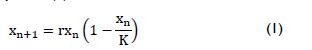
A dynamic system is one whose state changes as time elapses (Arrowsmith and Place, 1994). It is represented by a mathematical model (Campos and Isaza, 2002) which can be determined by difference equations, ordinary differential equations and stochastic differential equations. Such mathematical models are usually nonlinear and it is well-known that a nonlinear dynamical model can involve very complicated behaviour (Perko, 1991). A discrete system is a discrete logistic population growth model known as a logistic difference equation (Brauer and Castillo-Chávez, 2001), represented by equation (1):
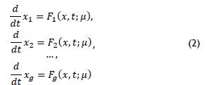
The change of state of a continuous dynamic system can be described by a set of first order differential equations (n=1,2,...,g) (Campos and Isaza, 2002), system (2):
The Runge Kutta 4th order numerical method (Mathews and Fink, 1999) is used to obtain a phase portrait and system solutions in the numerical simulation of such systems; Ramasubramanian and Sriram's method (Ramasubramanian and Sriram, 2000) is used for calculating Lyapunov exponents. A stochastic differential equation's general expression is given by equation (3), (Honerkamp, 1994):
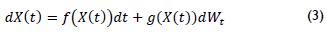
Euler-Maruyama and Milstein methods (Higham, 2001) are used for simulating such systems.
Software for analysing and simulating dynamic systems
Very few computational tools are currently available for simulating and analysing dynamic systems; some tools are complex in their use, requiring a commercial licence and are mostly developed just for a particular application.
Tools of this type would be the graphic bifurcation identifier (GBI) (Tovar, 2000), using MATLAB, which locates and identifies local bifurcations in discrete and continuous dynamic systems, autonomous and multiparametric dynamic systems and multidi-mensional dynamic systems. Its graphical interface is complicated for a user lacking MATLAB experience or without very detailed help on how to use the software. Java PHASER (Glick and Kocak, 2010) simulates discrete and continuous dynamic systems using real variables; its disadvantage lies in it being commercial software (Phaser Scientific Software, LLC) whose code is not available to a user and (obviously) is not free software (last released 2009). MATDS (Govorukhin VN, 2010) is MATLAB -based software for investigation of dynamic systems; it displays bifurcations and Lyapunov exponents, has few system analysis methods and its graphical interface is a bit complex to use. pplane and dfield (Polking and Arnold, 2010) generate and display a dynamic system's phase portraits and vector field. It has basic functions for simulating a system but it cannot fully analyse a dynamic system; it is found in versions for Java and MATLAB. MatCont (Govaerts and Kuznetsov, 2010) is a MATLAB graphics package for the interactive numerical study of dynamic systems, specialising in analysis of bifurcations. DDE-BITFTOOL (Luzyanina, Samaey, Roose and Verheyden, 2010) is a MATLAB package for numerical bifurcation and stability analysis of delay differential equations having delay of several fixed discrete and/or state dependent portraits. It enables computational analysis of steady-state solu-tion continuity and stability. System-Solver (Domínguez, Ardilla and Bustamante, 2010) is a free, open source tool for modelling dynamic systems in Java and focuses on the numerical solution of deterministic dynamic systems using the Runge-Kutta method; it only has that function but its advantage lies in solving systems of equations of any order and exporting data to other programming languages.
Compared to the aforementioned methods, DSamala toolbox is a complete tool because it has a variety of features, like its graphical user interface, which is very simple and easy to use and has a set of functions (toolbox) where the user can control the numerical code developed, thereby allowing better analysis and simulation of a dynamic system. DSamala toolbox can be used from the functions contained in the toolbox if a user has knowledge of MATLAB; if not, then through the graphical interface. This tool is complemented by a graphical interface manual and toolbox function reference manual. This software is free and can be downloaded from the MATLAB central repository at: http://www.mathworks.es/matlabcentral/fileexchange/27171-sdamala-toolbox
The DSamala toolbox thus represents a new alternative for software for teaching and research in the area of dynamic systems.
Methodology
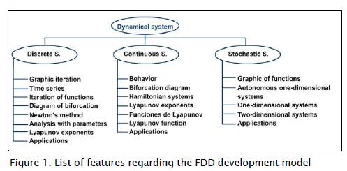
Feature driven development (FDD) was used for developing DSamala toolbox (Palmer and Felsing, 2002). The overall model fits dynamic systems which are broken down into three models: discrete, continuous and stochastic systems. Each has a list of features which are characteristics of the software (Figure 1):
Discrete systems
Graph iteration displays a discrete system's behaviour and is ana-lysed by returning fixed points and classifying them as being repeller, attractor or not hyperbolic. Time series graph a system's time series and returns values for such series. This graph shows whether a system has periodic points and their stability. Function iteration leads to obtaining fixed points for a selected period and the graph of their behaviour. A bifurcation diagram shows a graph observing changes in a system's dynamics (i.e. a parameterised family of functions where parameters vary). Newton's method is a basic tool for finding fixed points, graphically showing the value found as the method's convergence. Analysis with parameters analyses a parameterised system's dynamics. It establishes fixed points for the system in terms of parameters and may give these parameters values for generating graphical behaviour. Lyapunov exponents analyse system stability, thereby determining whether a system is chaotic; bifurcation points are obtained for a parameterised family. Applications interact with some default examples (logistic equation, Julia set and Mandelbrot set) where a user enters the data, simulation is performed and system behaviour observed.
Continuous systems
Behaviour involves simulating a system and phase portrait, solution curves, vector field, nullclinales and points of equilibrium, along with their respective classification. Bifurcation diagram shows changes in continuous system dynamics, parameterised as parameter value varies. Hamiltonian systems check whether a system is conservative; if so, the Hamiltonian function is obtained and its graph, together with contour lines. Lyapunov exponents give exact values, unlike discrete systems which only generate a graph of the evolution of these exponents as time elapses. Lyapunov function allows analysing system stability; it is essential when this cannot be done from behaviour functionality, for example, in the case of zero eigenvalues. Analysis with parameters allows analysing parameterised systems, indicating points of equilibrium and the type of behaviour. Application interacts with some default examples (Lorenz system or harmonic oscillator) where a user can enter data, simulate and observe system behaviour.
Stochastic systems
Graphic functions graph a stochastic function and can analyse systems in one and two dimensions. Autonomous one-dimensional systems graph this type of system's behaviour with constant deterministic functions. One-dimensional dynamic systems graph one-dimensional system's solution having any deterministic function. Two-dimensional systems plot 2D systems' phase portrait and solution curves. Applications interact with some default examples (Lotka-Volterra stochastic system and SI stochastic epidemic model) where a user can enter data, simulate and observe behav-iour.
Results
Installing the product
The DSamala toolbox was developed using MATLAB version R2009a. MATLAB version R2008a must be installed (or any higher version) for its operation with the image processing toolbox and symbolic math toolbox. The dsamala folder must be copied in a local file and added to the MATLAB path. The software can then be used via the graphical user interface by writing dsamala in the MATLAB command window or by using the functions contained in the command window toolbox or invoked from a MATLAB script.
DSamala toolbox structure
Figure 2 shows the general running of the DSamala toolbox graphical user interface; the type of dynamic system can be chosen (discrete, continuous or stochastic). The required functionality, data is then entered in the current application and output data displayed (a graph or data analysis of the selected system). This can be done as often as desired until is all active windows are closed.
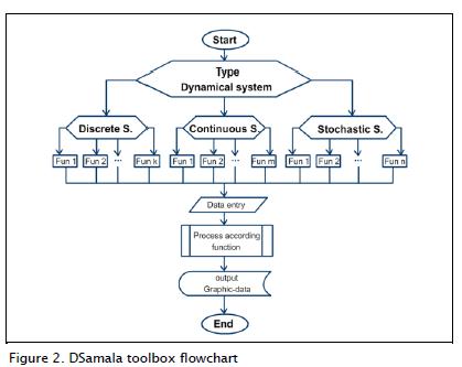
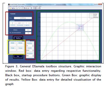
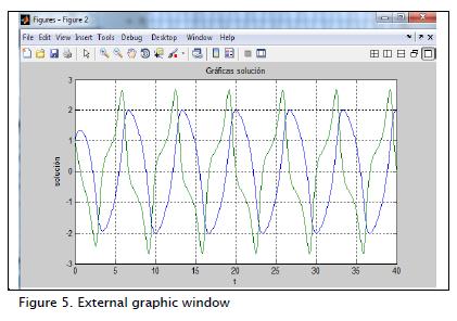
Figure 3 shows the DSamala toolbox graphical user interface. Additional windows are displayed for some features; for example, analysis output data is displayed in one window (Figure 4) and external figures in other windows (Figure 5). Function structure would be:
[exit_1,exit_2,...exit_m]=functionname(parameter_1,
parameter_2,...,parameter_n);
where exit_m means variables returned by a function called functionname having parameters parameter_n.
Use
A brief description of the main applications of discrete systems, continuous and stochastic menus, using GUI, is given below.
Discrete systems
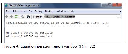
The logistic function is given by equation (1), r= 3.2. Figure 3 shows orbit, c= 0.3. The report window shown in Figure 4 indicates fixed point classification. Figure 6 shows a second itera-tion generated by graphical Iteration. Figure 7 shows the report of points from period two.
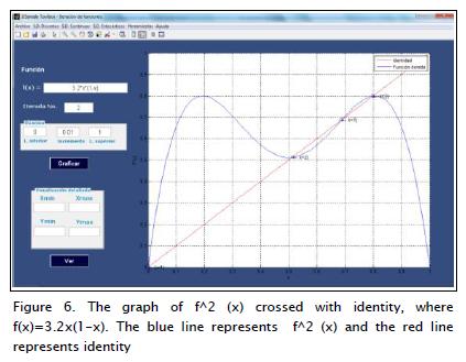
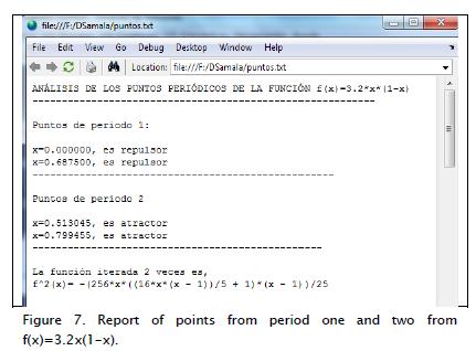
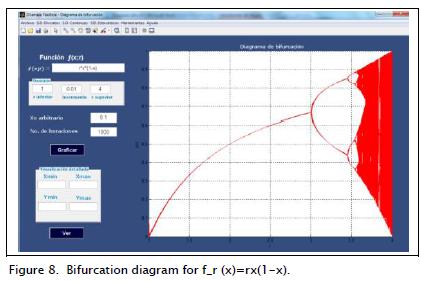
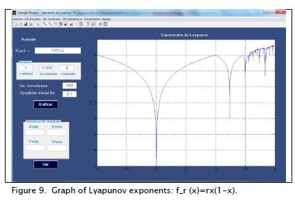
Figure 8 shows a diagram of parameterised family bifurcation for equation (1), showing changes in system dynamics as is varied from 1 to 4 (0.01 increase). Figure 9 shows the graph of the Lyapunov exponents of the logistic function, equation (1). The syntax for plotting the Lyapunov exponents shown in Figure 9 is:
[rr,lam]=td_explp(f,domr,Xo,nit)
Continuous systems
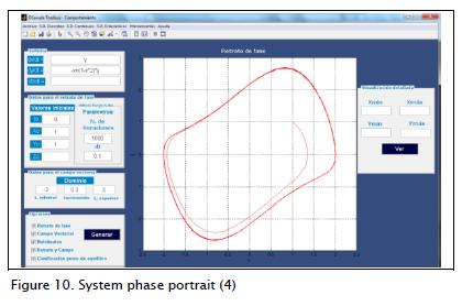
One-, two- or three-equation systems can be analysed and simulated. A well-known example would be the Van der Pol oscilla-tor, given by system (4):
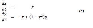
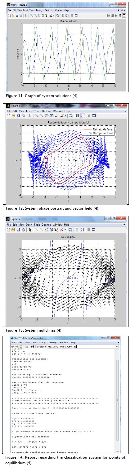
A phase portrait system (4) is shown in Figure 10. Other graphs are generated in external windows regarding system solutions, the phase portrait and vector field on one graph, the nullclines and a report of the classification of equilibrium points (Figures 11-14, respectively). The syntax for the main functions used in behaviour are:
- Portrait phase:
portrait1(f,x0,y0,dt,n)
[XX,YY,t]=portrait2(f,g,dt,x0,y0,t0,n)
[XX,YY,ZZ,t]=portrait3(f,g,h,dt,Xo,Yo,Zo,to,int)
- Vector field:
direction1(f,li,c,ls)
[dx,dy]=direction2(f,g,li,c,ls)
direction3(f,g,h,li,c,ls)
- Analysis of dynamic of the system:
clasduni(f,to,Xo)
clasdbi(f,g)
clasdtri(f,g,h)
- System solution and nulclinales: [solx,soly,solxg,solyg]=solution(f,g,xo,yo,to)
nullclines(f,g,dom)
where f, g and h are equations, xo, yo and zo initial variable values regarding initial time, n the number of iterations, (li)an interval defined by an initial value (c) an increase and(ls)a final value.
Figure 15 shows the Lyapunov exponents calculation regarding system time series (5); Figure 16 shows the report of exponents obtained for this system.

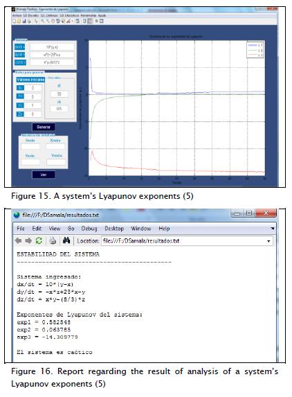
The syntax for calculating Lyapunov exponents is:
[T,Res]=tc_explyapunov(f,to,dt,tf,ystartutp)
[T,Res]=tc_explyapunov2(f,g,to,dt,tf,ystart,ioutp)
[T,Res]=tc_explyapunov3(f,g,h,to,dt,tf,ystart,ioutp)
where f, g and h represent equations, to the initial time, dt the increase of time, tf the final time, ystart the vector having initials conditions for variables x,y and z, ioutp the interval for showing data.
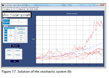
Stochastic systems
Figure 17 shows several operations and the average thereof, representing the solution of a one-dimensional stochastic dynamic system given by equation (6):

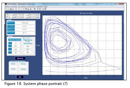
System (7) represents a stochastic population model:
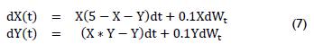
Figures 18 and 19 show the phase portrait and curve solution of system (7), respectively.
Conclusions
The Dsamala toolbox is a scalable, easy to use, open source tool which is available free online, gives accurate results and reduces costs regarding time and effort in the areas being studied. This tool is a new software alternative for studying and investigating discrete, continuous, stochastic dynamic systems.
DSamala provides added value for science education; a student can manipulate and control variables, make decisions and solve problems, thereby strengthening the training of research skills and scientific attitudes leading to more meaningful learning. The DSamala toolbox expands and deepens the scope of more tradi-tional science tools and instruments.
The tool's scope may be expanded using it for solving greater than 3rd order continuous systems and including more aspects regarding bifurcation study.
References
Arrowsmith, D.K., Place, C.M., Introduction to dynamical systems, Cambridge University Press, Cambridge, 1994. [ Links ]
Aubin, D., Dalmedico, A.D., Writing the history of dynamical systems and chaos: longue durée and revolution, disciplines and cultures, Historia Mathematica, 29, 2002, pp. 1-67. [ Links ]
Brauer, F., Castillo-Chávez, C., Mathematical models in population biology and epidemiology, Texts in Applied Mathematics, 40, Springer, New York, 2001. [ Links ]
Brin, M., Stuck, G., Introduction to dynamical systems, Cambridge University Press, USA, 2003. [ Links ]
Campos, D., Isaza, J.F., Prolegómenos a los sistemas dinámicos, Universidad Nacional de Colombia, Bogotá, 2002. [ Links ]
Cellier, F.E., Kofman, E., Continuous systems simulation, Springer, New York, EEUU, 2006. [ Links ]
Domínguez, E., Ardilla, F., Bustamante, S., System-Solver: Una herramienta de código abierto para la modelación de sistemas [ Links ]
Govaerts W., Kuznetsov Y., MatCont. [Online]. [Access date: May 12th 2010]. Available at: http://www.matcont.ugent.be/ [ Links ]
Glick, J., Kocak, H., Phaser. [Online]. [Access date: April 10th 2010]. Available at: http://www.phaser.com/ [ Links ]
Govorukhin, V.N, MATDS. [Online]. [Access date: April 18, 2010]. Available at: http://www.math.rsu.ru/mexmat/kvm/matds/ [ Links ]
Higham, D.J., An algorithmic introduction to numerical simulation of stochastic differential equations, SIAM Review, Vol. 43, No.3, 2001, pp. 525-546. [ Links ]
Holmgren, R.A., First course in discrete dynamical systems, Springer-Verlag, New York, EEUU, 1996. [ Links ]
Honerkamp, J., Stochastic dynamical systems concepts, numerical methods, data analysis, Wiley, 1994. [ Links ]
Kuznetsov, Y.A. Elements of applied bifurcation theory (3rd Edition). Appl. Math. Sci., 112. Springer-Verlag, New York, 2004. [ Links ]
Lorenz, E.N., Deterministic nonperiodic flow, Journal of the Atmospheric Sciences, 20, 1963, pp. 130-141. [ Links ]
Mandelbrot, B.B., Fractals and chaos: the mandelbrot set and beyond, Springer-Verlag, New York, 2004. [ Links ]
Mathews, J., Fink, K., Numerical methods using MATLAB, Third Edition, Prentice Hall, 1999. [ Links ]
Palmer, S.R., Felsing, J. M., A Practical guide to feature-driven development, Prentice Hall, Estados Unidos, 2002. [ Links ]
Perko, L. Differential equations and dynamical systems, Springer, Berlin, 1991. [ Links ]
Polking, J., Arnold D. pplane and dfield. [Online]. [Access date: March 21, 2010]. Available in: http://math.rice.edu/~dfield/dfpp.html [ Links ]
Ramasubramanian, K., Sriram, M.S., A comparative study of computation of Lyapunov spectra with different algorithms, Journal of Physica D., Vol 139, 2000, pp 72-86. [ Links ]
Strogatz, S.H., Nonlinear dynamics and chaos, with applications to physics, biology, chemistry and engineering, Perseus Books, New York, 1994. [ Links ]
Tovar, A. Herramienta para la detección de bifurcaciones locales en sistemas dinámicos no lineales, MSc thesis, Universidad Nacional de Colombia, Bogotá, 2000. [ Links ]

