J. D. Rairán Antolines¹

¹ José Danilo Rairán Antolines. Ingeniero Electricista, Universidad Nacional de Colombia, MSC Computer Science, Universidad Nacional de Colombia. Affiliation: Universidad Distrital Francisco Jose de Caldas, Colombia. E-mail: drairan@udistrital.edu.co

How to cite: Rairán, J. D., An optimal algorithm for estimating angular speed using incremental encoders., Ingeniería e Investigación. Vol. 33, No. 2. August 2013, pp. 56 - 62.

ABSTRACT

This paper proposes a new algorithm using signals from an incremental encoder for estimating a rotating shaft's speed. This algorithm eliminated the oscillations appearing in classical fixed-time and fixed-space algorithms, even when speed was constant. A fixed-time algorithm measures angular displacement at fixed-time intervals, while a fixed-space algorithm measures time every fixed-angular displacement. Time and displacement measurements were used to generate estimations for speed. The new algorithm generated a unique value for estimating speed due to synchronising encoder pulses and a signal formed by impulses every time increase (delta). A first modification of the proposed algorithm was defined, resulting in the harmonic mean between these two proposed alternatives having the smallest relative error possible. This error was always smaller than half the error with fixed-time and fixed-space algorithms. Experimental setup and algorithms are shown, as well as Simulink results using signals acquired from an incremental encoder.

Keywords: Fixed-space, fixed-time, incremental encoder, optimal algorithm, estimating speed, truncation error.

RESUMEN

En este artículo se propone un algoritmo nuevo, el cual utiliza las señales provenientes de un encoder incremental para aproximar la velocidad de giro de un eje. Este algoritmo elimina las oscilaciones que aparecen en los algoritmos clásicos, conocidos como a espacio fijo y a tiempo fijo, las que son visibles incluso a velocidad constante. Un algoritmo a tiempo fijo mide desplazamiento angular a intervalos de tiempo fijo, mientras que un algoritmo a espacio fijo mide tiempo a intervalos de espacio fijo. Las medidas de tiempo y desplazamiento se utilizan para estimar la velocidad. El algoritmo nuevo genera una aproximación sin saltos a velocidad constante, dada la sincronización entre los pulsos del encoder y la señal formada a partir de impulsos cada delta de tiempo. Se propone una primera modificación del algoritmo, y el resultado es que el promedio armónico entre las dos propuestas de algoritmo tiene el menor error relativo posible. Ese error siempre es menor que la mitad del error que se produciría con los algoritmos a tiempo fijo o a espacio fijo. Finalmente, se presenta un arreglo experimental para probar los algoritmos, y se muestran los resultados de la ejecución en Simulink, usando señales adquiridas de un encoder incremental.

Palabras clave: Aproximación de la velocidad, error de truncamiento, espacio fijo, tiempo fijo.

Received: May 31st 2012 Accepted: July 19th 2013

Introduction

Estimating speed represents an interesting problem, especially regarding control involving the dynamics of a system based on signals given by sensors; i.e. based on an estimations of what actually happens. The algorithm proposed in this paper was aimed at obtaining maximum information from an incremental encoder, thus establishing a fast and stable measurement of a shaft's angular speed. An incremental encoder is an electromechanical instrument. The mechanical part is an evenly spaced slotted disc, whereas the electric part includes a light beam and detector. A high light level (one) is recorded when the light passes through the slit and reaches the detector, and zero otherwise.

Measuring speed has one physical limitation; estimating speed requires measuring two instants in time and the result necessarily neglects one of them. An estimation of speed has at least two sources of error because it requires two measurements: position and time. Since ω_m is Δθ/Δt, error regarding estimation ω_m lies in the nature of such deltas (i.e. discrete and digital values). Digital measurement involves an inevitable truncation error. Thus, Δθ is an integer multiple of the pulses emitted by the encoder (pul), and dt is likewise an integer multiple of clock resolution (ts).

The speed at which the time between two consecutive pulses from the encoder lasts exactly dt defines the so-called speed limit given in revolutions per second (ω_lim = (1/pul)/dt). Speed values less than ω_lim are low, whereas greater or equal than this are high. A similar concept (Tsuji et al., 2009) has defined what authors call speed resolution.

Two classical algorithms estimate speed (fixed-time and fixed-space algorithms); other algorithms usually come from these two. If an estimation involved using the fixed-time approach, which means updating the counting of pulses (Nep) each dt, then the algorithm generates an estimation ω_m = Nepω_lim. On the other hand, the fixed-space approach updates dt counts (called Ndt) between every two consecutive pulses, so ω_m = (1/Ndt)ω_lim. The fixed-space algorithm is recommended for low speeds, whereas the fixed-time algorithm is useful for high speeds. The truncation error makes ω_m oscillate regardless of the approach adopted. The effect of these oscillations requires using low-pass filters to smooth the value of the estimation, thereby implying delay.

Current solutions for avoiding the effect of truncation can be classified mainly into two groups: highly accurate measurements of time and synchronising position and time signal (a third group is also referenced, including other options). Solutions from the first group use the power of computing electronic circuits for high resolution measurement of time, for instance microcontrollers (Petrella and Tursini, 2008), DSP (Boggarpu and Kavanagh, 2010) and FPGAs. A more elaborate solution (Merry, Molengraft and Steinbuch, 2007) detects rising edges from the encoder to make a polynomial fitting, thereby smoothing the estimation. Other work (Lygouras et al., 2008) has gone so far as to claim that the truncation error effect disappears when clock resolution reaches 50 ns. The oscillations within the estimation, though small, still remain in this first solution group. On the other hand, the second group looks for synchronising position and time measurementents. An algorithm named the S method (Tsuji et al., 2009) has been proposed based on this synchronisation concept, mainly being helpful for high speed. Another proposal (Se-Han, Lasky and Velinsky, 2004) for optimising encoders with few slits uses synchronisation for high speeds, whereas for low speeds it switches the algorithms for another based on its model of the system. The third group of solutions is not exactly focused on the truncation problem, but nonetheless the problem is well referenced and is taken into account in the solution. Some work (Su et al., 2005) has focused on very low speeds, estimation being made by absolute position measurement while the average speed of every rotation (Hachiya and Ohmae, 2007) has been used for developing a simple and effective method for eliminating fluctuations, as well as mitigating the effect of some mechanical errors. Another solution consists of using filters and switching from fixed-time to fixed-space methods or vice versa to ensure obtaining the smallest relative error possible (D'arco, Piegari and Rivo, 2003). It has been suggested that some steps can be traced backwards to control the highest relative error (Liu, 2002).

Describing the new algorithm

The new algorithm presented in this section eliminated oscillations in estimating speed when they came from discrete and digital measurements, as in an incremental encoder. The core of the proposal consisted of synchronizing position and time pulses. Since there was no control over the time at which the encoder pulse appeared, the algorithm simply started to count dt when a position pulse appeared. As a result, such estimation would have been constant for constant speeds, without the use of state observers or system models as required in other work (Se-Han, Lasky and Velinsky, 2004).

Guaranteeing the mathematical results in this section involved the following assumptions: the encoder did not lose pulses during counting, measuring time was exact and in multiples of clock time (ts) and the mechanical distance between pulses remained constant. These assumptions idealised an incremental encoder's true performance, although they were necessary for ensuring error bounds on the estimations.

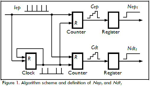
The first step in transforming the encoder signal detected the rising edge from each pulse. This detection generated a pulse train (Iep) as shown in Figure 1. The next step counted these pulses and led to a stair-type signal named (Cep). If counting Cep went to zero, for instance because the time reached dt, then a register saved the last value in the counter into a variable Nep1. The scheme in the lower part of Figure 1 illustrates an additional series of blocks. These blocks counted dts. A pulse dt resulted when the accumulation of ts reached the value of dt. This event reset and started the counting of ts over again. The counter block held dt counting in a variable Cdt. If an Iep pulse reset that counter, then a register held the last value of Cdt into Ndt₁.

Speed was estimated as ω_m1 = n₁ω_lim, where n₁ was Nep1/Ndt1. Counting required that Nep1 should be a whole number (0, 1, 2,...), while Ndt1 had to be a natural number. There were more Iep pulses in the count than dt pulses for speeds higher than ω_lim, so Ndt1 stayed fixed at one. On the contrary, there were more dt pulses than Iep pulses for speeds lower than ω_lim, so Nep1 remained fixed at one. Possible values for n₁, for high speeds were 1, 2, 3, and so on, and 1/2, ?, 1/4, and so on for low speeds.

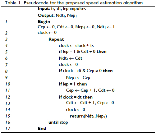
Table 1 shows the algorithm's pseudocode. This algorithm generated a new estimation ω_m1 every ts by computing Ndt1 and Nep1. The core of the algorithm synchronised time and space pulses in line 6 where the clock went to zero. However, this synchronisation did not mean that Ndt1 and Nep1 updated their values synchronously: Ndt1 updated its value in line 6 (synchronised with Iep pulses) and Nep1 updated its value in line 9 (synchronised with dt pulses).

Plots a) and b) in Figure 2 illustrate algorithm operation for low and high speeds, respectively. Event a started the programme in both examples, and subsequent letters defined other events. For instance, events d and g updated Nep1 in both examples. Estimation wm1 remained constant for events later than f in plot a. On the other hand, estimation after any event later than d in plot b remained constant.

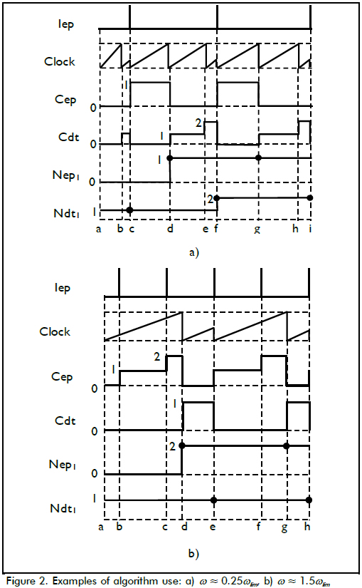
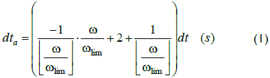
Solid points in Figure 2 depicted the time when the algorithm updated Nep1 or Ndt1. The time between updates for low speeds was dta = (ω_lim/w) dt, and for high speeds dta (see Eq. 1). The maximum value of dta in Equation 1 was twice dt as speed approached ω_lim, and delay decreased as w grew, with dt as its limit:

The value of Nep1 represented the ceiling for the number of pulses Iep, as can be seen in Figure 2; Ndt1 was the floor for counting dts, so estimation n₁, defined as Nep1/Ndt1, was always greater than the actual speed, as shown in Figure 3, where the X and Y axes had been scaled by ω_lim.

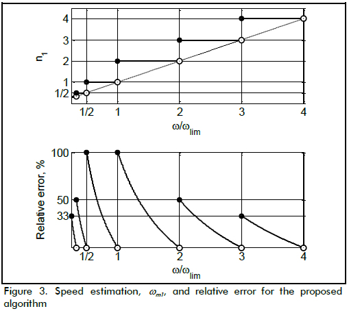
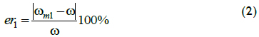
The first measurement of quality for estimating speed correlated relative error and speed, as shown in the lower part of Figure 3. A second measurement of quality (maximum relative error per interval) took into account that the value of w actually was unknown. An interval covered the whole range of speeds having the same estimation. For instance, all speeds estimated as n₁ = 3 as estimation defined an interval. This second measurement of quality depended entirely on algorithm output. Even so, Equation 2 showed the definition of relative error for the second measurement of quality to come up with an equation for this indicator:

Since ω_m1 = n₁ω_lim then,

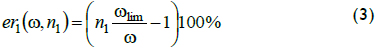
Relative error er₁ maximised its value at the left of each interval when ratio wlim/w was maximum. For high speeds (when n₁ exceeded 1), ratio wlim/w was the inverse of n₁ - 1, as can be seen by analysing the upper part of Figure 3. For instance, if n₁ = 3, maximum ratio would have been wlim/w = 1/2, so maximum relative error reached 50%. For low speeds the ratio was wlim/w = (1/n₁) + 1. For instance, if n₁ = 1/2, then wlim/w = 3, so maximum relative error reached 50% again. Previous analysis of ratio wlim/w produced the expression for the maximum relative error shown in Equation 4:

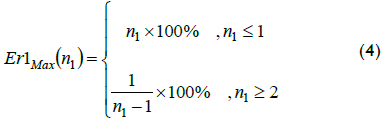
The relative error in Equation 4 matched the maximum relative error for the traditional fixed-time algorithm if w ≥ wlim and dt = ts. Er1_Max matched the maximum relative error for the traditional fixed-space algorithm, when w < ω_lim and dt = ts. The proposed algorithm equated its measurement of quality with relative error from traditional algorithms.

Optimising maximum relative error

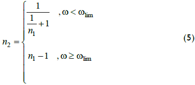
The algorithm's optimum minimised error Er_Max, such minimisation coming from an observation about where maximum error happened; according to the result shown in Figure 3, such maximum error took place at the left end from each interval. If the estimations shifted down one place, for example from n₁ equal to 3 to a new n₂ equal to 2, or from n₁ = 1/2 to n₂ = ?, then relative error decreased. This decrease occured due to the maximum difference between w and the new ω_m2 taking place at the right of each interval, instead of at the left.

The new estimation (ω_m2 = n₂ω_lim) requires n₂ as given in Eq. 5.

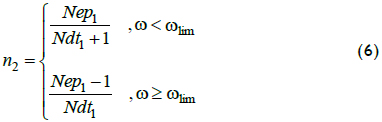
Nep₁ and Ndt₁ provide an alternate means for calculating n₂, as shown in Equation 6:

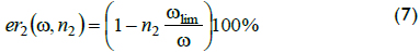
The relative error for estimation ω_m2 is shown in Equation 7:

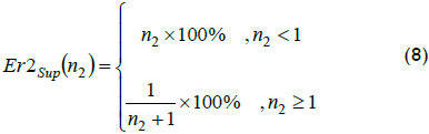
According to Equation 7, and for high speeds, every integer ratio w/wlim = n₂ + 1 maximised relative error. For instance if n2 equal to 2, then wlim/w was 1/3, so the maximum relative error reached 33.3%. For low speeds, integer ratio w/wlim was the inverse of (1/n₂) + 1. So, for instance, if n₂ = 1/2, fraction wlim/w = 3. As a result, maximum error reached 33.3% again. Error in terms of n₂ is shown in Equation 8. This equation defined a supremum and not a maximum, because the right end of each interval was open, as shown in Figure 3:

Computing estimation ω_m1 and ω_m2 required the actual value of w to classify a speed as low or high (Eq. 5 and 6). The value of the speed was unknown, although there were two approaches for determining whether speed passed speed limit, ω_lim. Both approaches used an indirect measurement. In the first approach, whereas low speeds had the time between consecutive Iep's exceeding dt, that time did not exceed dt for high speeds. The second approach counted n₁. Whereas that number exceeded n₁ ≥ 2 for high speeds, for low speeds it did not.

Estimation ω_m2 reduced maximum error by up to 50% with estimation ω_m1, mainly for speeds close to ω_lim. On the other hand, Er1_Max and Er2_Sup became closer and closer as speed went farther from ω_lim, or, in other words, when n₁ and n₂ went either to zero or infinity.

Any estimation greater than ω_m1 generated errors larger than Er1_Max; any estimation under ω_m2 resulted in errors over Er2_Sup. So if there was a way to reduce maximum error per interval, the resultant estimation would have fallen between ω_m1 and ω_m2. See, for instance that estimation ω_m3 equalled n₃ω_lim in Figure 4. The work then involved finding a value for n3 that minimised error in region ω_m2 ≤ ω_m3 ≤ ω_m1:

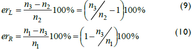
The minimum relative error for ω_m3 could have been on the right or left side at each interval. If estimation ω_m3 decreased, relative error on the left also decreased. As a result, relative error on the right increased. Thus, errors on the left opposed errors on the right and optimal value levelled the error on both sides, as shown by Equations 9, 10 and 11:

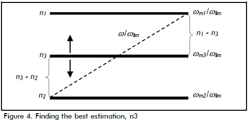
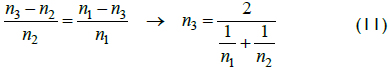
Error er_L reached zero when n₃ = n₂ in Equation 9, and according to the representation in Figure 4 the maximum occurred when n₃ equalled n₁. Equation 10 showed that erR reached zero when n₃ equalled n₁, and the maximum occurred when n₃ = n₂. Since er_R and er_L were linear, then the minimum from combining er_R and er_L occurred when er_L equalled er_R, as shown in Equation 11. The value of n₃ in Equation 11 defined optimal estimation for ω_m3: the harmonic mean between ω_m1 and ω_m2. No other value of n_i produced a smaller error:

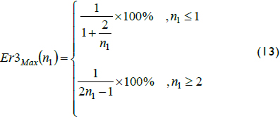
Error Er3_Max was defined in terms of n₃ in Eq. 12, and in terms of n₁ in Eq. 13:

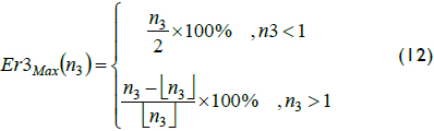
If n₁ = 1 or 2 in Equation 13 then Er3_Max equalled one third of the error given by Equation 4. On the other hand, when n₁ → ∞ or n₁ → 1/∞ then error Er3_Max went below half Er1_Max. Therefore, this third estimation ω_m3 in fact optimised error by setting the smallest possible bound for the relative error at each interval.

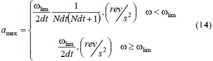
The bounds for relative error were calculated for constant speed and also applied to variable speeds, if acceleration did not go beyond a given bound. The method for finding the maximum acceleration began by supposing constant acceleration and high speeds. Under these assumptions, and according to the result in Equation 1, any estimation wmi updated its value at most every 2dt, so maximum acceleration had an increase in speed equal to ω_lim in an interval of time equal to 2dt. The same analysis could be made for speeds under ω_lim, as shown in Equation 14:

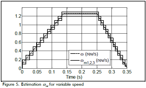
The solid lines in Figure 5 illustrate estimations wmi, and the dashed line represents the actual speed. Estimation ω_m1 was always greater than ω_m3, and ω_m3 was always greater than ω_m2. The simulation parameters in Figure 5 were dt = 1 ms, pul = 10,000 and ts = 0.1 ms. These values made ω_lim = 0.1 rev/s, so maximum acceleration was amax = 50 rev/s². The ramp with positive acceleration had 8.33 rev/s² constant acceleration whereas negative acceleration was -12.5 rev/s².

The estimation technique tested in this section was also used as an incremental encoder, so the results appeared to be limited to measuring angular speed, even though this technique can be equally applied for estimating any variable's rate of change. There was only a single restriction on the data: sampling rate had to be constant. This restriction, along with the discrete nature of the measurements, generated oscillations on traditional estimation algorithms, even when the rate of change remained constant; however, those oscillations disappeared when using the proposed algorithm.

Experimental results

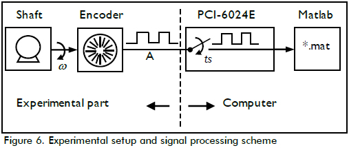
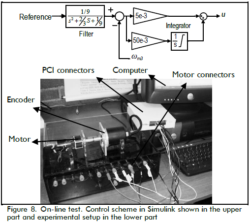
In this section, the algorithm generated estimations using real signals coming from an encoder. The scheme in Figure 6 illustrates an encoder coupled to a shaft, where the system aimed at estimating the shaft's angular speed. The encoder's output fluctuated from zero to five volts for low and high levels, respectively. A data acquisition card captured this voltage signal, and a computer recorded its values for later use. Data acquisition card PCI-6024E had 100 ms ts sampling time. The 160-slot encoder and the DC motor (Minertia 6GFMED) are shown in the lower part of Figure 8.

The algorithm's verification required an actual value of w to compute relative error. Instead of using a highly accurate sensor for obtaining the aforementioned value, the proposed algorithm found estimations using the best parameters for the smallest feasible error. For instance, ideal parameters were pul = 160 and dt = 2 s. These parameters guaranteed a boundary for relative error = 0.07%, when w = 2 rev/s, as shown in Equation 12. This error decreased to 0.0065%, if w equalled 24 rev/s.

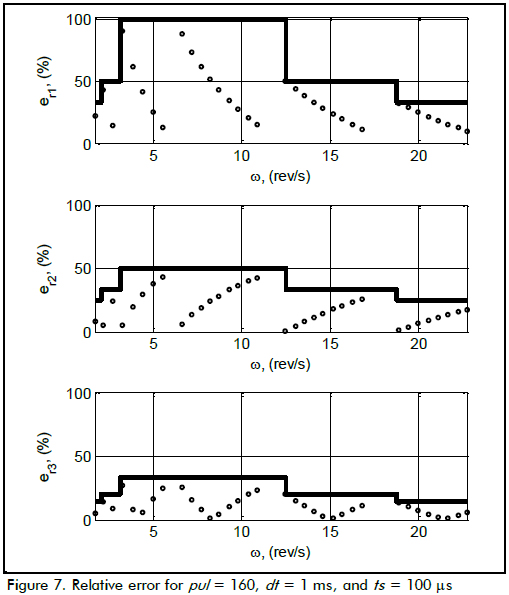
The first experiment had the next parameters: pul = 160 and 1 ms for dt, dt thus overcoming ts by a factor of ten. In order to capture the data, the motor ran at constant voltage; a computer then saved data for ten seconds starting only when the motor entered its stationary stage. The algorithm obtained estimations using the recorded data as input. The same steps were repeated every 0.5 V for constant voltages from 3 to 24 V.

The solid line in Figure 7 represents the bound for relative error per interval, as indicated in Equations 4, 8 and 13. The dots represent the experimental values for relative errors: er₁ for ω_m1, er₂ for ω_m2 and er₃ for ω_m3. Results in Figure 7 agreed with the analysis given in the previous section. Relative errors always fell within bounds, and estimation ω_m3 consistently had minimum relative error.

Other experiments have used dt equal to 2, 5, 10, 20, 50 and 100 ms. If dt increased ω_lim decreased. For instance if dt were greater than 5 ms, ω_lim went below experimental shaft speed. The greater the dt, the larger the n_i and, as a result, relative error decreased, but updating time increased. So the relationship between dt and relative error became a trade-off problem, the solution of which depended on its application.

Relative error also decreased by making ω_lim higher than any experimental speed; this change in ω_lim value required the use of an encoder having a lower number of slots, or the definition of a smaller dt. Thus, instead of changing the encoder to run this experiment, only one of every k pulses of the encoder was recorded. The experiment used k = 40 and dt = 1 ms. So ω_lim = 250 rev/s, and since all speeds fell under 30 rev/s, maximum relative error fell under 10%, as was experimentally proven.

The algorithm was tested on-line using an embedded system for testing the algorithm's application in an electronical device (i.e. dsPIC33FJ128MC802). dsPIC output was estimated as ωm3, closing a control loop in Simulink, as shown in the upper part of Figure 8, where u was the actuating signal. The filter made the system slow enough to have ts = 1 ms and dt = 40 ms.

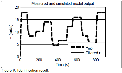
Identification involved using the filtered reference as input and ωm3 as ouput. The identification result is shown in Figure 9. The model for the output-input ratio, H(S), was H(S) = 1/((1+1.512S)(1+1.506S)). The model fit 94.41% of the data after 20 iterations, thereby showing the quality of the data and control loop.

Conclusions

A new algorithm for estimating speed has been proposed proven and experimentally tested (using incremental encoders). One of the the algorithm's advantages was that it had constant output when the speed was constant, contrary to fixed-time and fixed-space algorithms producing two values.

Relative error for the stationary case was computed and compared to fixed-time and fixed-space algorithms, showing that maximum relative error per interval was the same, where an interval was defined as the range of speeds havin the same value as estimation. A modification of the algorithm has been proposed, aimed at reducing maximum relative error by interval. It was proved that the optimal value was the harmonic mean between estimation ω_m1 and ω_m2. The maximum relative error was always smaller than half of that produced by fixed-time and fixed-space algorithms.

Even when the mathematical proof was made for constant speed, it was shown that the estimation remained valid for acceleration smaller than a given maximum, depending exclusively on pul and dt for high speed and pul, dt and Ndt for lower speed.

Observing experimental data showed the effect of changing parameters dt and pul in the encoder; such parameter changes reduced the relative error of the estimation, and could be done using three approaches: increasing pul and dt at their highest possible values, reducing pul and dt and decreasing ts.

Some problems of interest remain. For example, it appears that an adaptive algorithm for dynamically changing the value of dt, ts and k could boost algorithm performance, because making ω_lim greater or smaller than current speed would reduce error in the estimation. Implementing the algorithm in an embedded system, faster than dsPIC, including additional aspects such as rotation sense (also called sign) would make the algorithm ideal for use in industrial applications.

References

Boggarpu, N., Kavanagh, R., New Learning Algorithm for High-Quality Speed Measurement and Control When Using Low-Cost Optical Encoders., IEEE Trans. on Instrumentation and Measurement, Vol. 59, No. 3, Mar., 2010, pp. 565-574.         [ Links ]

D'arco, S., Piegari, L., Rivo, R., An Optimized Algorithm for Speed Estimation Method for Motor Drives., Proc. Symposium on Diagnostics for Electric Machines, Power Electronics and Drivers, Atlanta, GA, USA, Aug., 2003, pp. 76-80.         [ Links ]

Hachiya, K., Ohmae, T., Digital speed control system for a motor using two speed detection methods of an incremental encoder., Proc. European Conference Power Electronics and Applications, Aalborg Denmark, 2007, pp. 1-10.         [ Links ]

Liu, G., On speed estimation using position measurements., Proc. American Control Conference, Anchorage, Alaska, USA, 2002, pp. 1115-1120.         [ Links ]

Lygouras, J., Pachidis, T., Tarchanidis, K., Kodogiannis, V., Adaptive High-Performance Speed Evaluation Based on a High-Resolution Time-to-Digital Converter., IEEE Trans. on Instrumentation and Measurement, Vol. 57, No. 9, Sep., 2008, pp. 2035-2043.         [ Links ]

Merry, R., Molengraft, R., Steinbuch, M., Error modeling and improved position estimation for optical incremental encoders by means of time stamping., Proc. 2007 American Control Conference, New York City, USA, 2007, pp. 3570-3575.         [ Links ]

Petrella, R., Tursini, M., An Embedded System for Position and Speed Measurement Adopting Incremental Encoders., IEEE Trans. on Industry Applications, Vol. 44, No. 5, Sep., 2008, pp. 1436-1444.         [ Links ]

Se-Han, L., Lasky, A., Velinsky, S., Improved Speed Estimation for. Low-Speed and Transient Regimes Using Low-Resolution. Encoders., IEEE/ASME Trans. on Mechatronics, Vol. 9, No. 3, Sep., 2004, pp. 553-560.         [ Links ]

Su, Y. X., Zheng, C. H., Sun, D., Duan, B. Y., A Simple Nonlinear Speed Estimator for High-Performance Motion Control., IEEE Trans. on Industrial Electronics, Vol. 52, No. 4, Aug., 2005, pp. 1161-1169.         [ Links ]

Tsuji, T., Hashimoto, T., Kobayashi, H., Mizuochi, M., Ohnishi, K., A Wide-Range Speed Measurement Method for Motion Control., IEEE Trans. on Industrial Electronics, Vol. 56, No. 2, Feb., 2009, pp. 510-519.         [ Links ]