J. Carrillo¹, A. Rubiano² and A. Delgado³

¹ Julian Carrillo. PhD in Structural Engineering. Affiliation: Researcher and Professor, Universidad Militar Nueva Granada, UMNG, Colombia. E-mail: wjcarrillo@gmail.com

² Astrid Rubiano. MSc in Engineering. Affiliation: Researcher and Professor, Universidad Militar Nueva Granada, UMNG, Colombia. E-mail: astrid.rubian@unimilitar.edu.co

³ Arnoldo Delgado. MSc in Engineering. Affiliation: Researcher and Professor, Universidad Militar Nueva Granada, UMNG, Colombia. E-mail: arnoldo.delgad@unimilitar.edu.co

How to cite: Carrillo, J., Rubiano, A., Delgado, A., Evaluation of Green's function when simulating earthquake records for dynamic tests., Ingeniería e Investigación, Vol. 33, No. 3, December 2013, pp. 28 - 33.

ABSTRACT

When dynamic performance of structures is assessed experimentally, most experimental studies consider variation in intensity by increasing the record of peak ground acceleration or displacement at different values. However, severity of earthquake motion is not only a function of the concerns instrumental intensity, but also the frequency content, duration and the amount of energy imposed on the structure. To fulfill dynamic test conditions, this paper describes and discusses a novel method for selecting several seismic events characterising the seismic area and fulfilling particular similitude requirements. The method included using an earthquake record as an empirical Green's function for simulating larger magnitude events. Three seismic events used for shake table testing of reinforced concrete walls for low-rise housing are presented and discussed to validate the proposed method's results.

Keywords: Green's function, earthquake record, shake table test, similitude requirement.

RESUMEN

Cuando se evalúa experimentalmente el desempeño dinámico de las estructuras, la mayoría de estudios consideran la variación de la intensidad a partir del incremento del registro, hasta los diferentes valores de la aceleración o del desplazamiento máximo del mismo. Sin embargo, la severidad del movimiento sísmico es una función no sólo de la intensidad instrumental, sino del contenido de frecuencias y de la cantidad de energía impuesta sobre la estructura. Para cumplir las condiciones dinámicas del ensayo, el artículo describe y discute un nuevo método para seleccionar varios eventos símicos, que caracterizan la zona sísmica y que cumplen con requisitos particulares de similitud. El método incluye el uso de un registro sísmico como una función empírica de Green para simular eventos de mayor magnitud. Para validar los resultados del método propuesto, se presentan y discuten tres eventos sísmicos que fueron utilizados para ensayos en mesa vibratoria de muros de concreto reforzados para vivienda de baja altura.

Palabras clave: función de Green, registro sísmico, ensayo en mesa vibratoria y requisitos de similitud.

Received: November 22th 2012 Accepted: July 26th 2013

Introduction

Experimental programs usually involve testing several specimens; they should be tested under similar conditions when comparing response. An experimental program could involve a test method where the time scale of record is individually modified for testing each specimen (Dowling, 2006). It would thus be unfeasible to compare specimen performance by using the level of seismic intensity because the duration of the record used for each specimen is different.

A novel method to fulfill dynamic test conditions is proposed in this study. It consists of selecting several seismic events characterising the seismic area and fulfilling particular similitude requirements. Considering that earthquake motion records are the main source for testing structures under dynamic loading, it is proposed that an earthquake record be considered as an empirical Green's function for simulating larger magnitude events. Ground-motion simulation using stochastic summation of small earthquakes is implemented for defining seismic demand.

Seismic events for shake table testing of reinforced concrete walls for low-rise housing are presented and discussed to validate the proposed method's results. Seismic events were associated with limit states and therefore three earthquake hazard levels were selected. A M_W 7.1 was used for seismic demand representing diagonal cracking limit state. The M_W 7.1 record was considered a Green's function for simulating larger magnitude events. Two earthquakes having magnitudes M_W 7.7 and M_W 8.3 were numerically simulated for the strength and near-collapse limit states, respectively.

Dynamic requirements for shake table tests

Three objectives should be established for shake table tests of all specimens included in an experimental program. The first goal is to fulfill dynamic similitude between specimens by establishing a similar period ratio for each specimen; period ratio is defined as the ratio between the periods of vibration of the specimen and the dominant periods of the earthquake spectrum. Second objective is to achieve the specimen's damage under conditions close to dynamic resonance; this occurs when the period of the specimen is located in the range of dominant periods of earthquake spectrum. Third goal is to compare specimen response in terms of seismic intensity by unchanging record duration and thus the record used for all specimens should be the same at a certain level of seismic intensity.

A test method can be used to achieve the first two objectives where the records' time scale is individually modified when testing each specimen. The scale factor is calculated so that the period ratio is identical when testing each model (Dowling, 2006). Testing all specimens using this method is carried out in conditions close to dynamic resonance. However, specimen performance cannot be compared by using the level of seismic intensity because the duration of the record used for each specimen is different. In addition, the shake table system capacity could be lower than that needed for reproducing the time scale calculated for achieving the period ratio. Moreover, data post-processing would be time-consuming.

A novel method consists of selecting seismic events characterising the seismic area and fulfilling particular requirements. For instance, the range of periods having higher spectral intensities should be similar to the range of periods of vibration of the specimens during all testing stages. In addition, spectral intensity variation should be minimal within the specimens' range of periods for each seismic event. The earthquake record time scale would not have to be modified and thus specimen response could be compared in terms of seismic intensity level.

Green's function for simulating earthquakes

Named after the British mathematician George Green who first developed the concept in the 1830s, Green's function enables solving inhomogeneous differential equations subject to specific initial conditions (Li, 2012). In linear elastodynamics, the displacement time field due to a unit impulsive point load, precisely defined in both space and time, is called Green's function. The displacement-time field due to the same type of load at the same location, acting for a finite time, can be found by convolution of Green's function (Koller et al., 1996).

Estimation of future ground motion at a given site from a postulated earthquake of known magnitude is a basic problem for seismologist and structural engineers. Theoretical calculations may lead to unreliable time history, especially at high frequencies, since the crustal structure and local site effects are poorly known at the required wavelengths. An attractive alternative, originally proposed by Hartzell (1978), is to use small earthquake recordings as empirical Green's functions. Since such recordings inherently include propagation and site effects, uncertainties associated with crustal structure and local geology are eliminated, provided that small earthquake recordings sample the target event's entire fault plane. This requirement is often not met, since only a few recordings are available to be used as suitable Green's function. Both theoretical and empirical Green's function techniques, however, require rupture specification (Ordaz et al., 1995).

Basis of the empirical Green's function

The basic idea behind the method of the empirical Green's function is to interpret the instrumentally measured response to a small seismic event as an empirical Green's function and convolute it suitably to simulate response to a large earthquake. Many scientists have further developed Hartzell's idea. The empirical Green's function is taken at several times and added so that a larger earthquake of the same focal mechanism and hypocentre is synthesised. The repeated small events are thought to be distributed over a hypothetical fault whose size is that expected for a larger earthquake (the "target" event). Time delays are introduced between the repeated events roughly simulating a physically realistic rupture process across the hypothetical fault. The number of added events and the summation are reduced from scaling relationships of source parameters and scaling laws between earthquakes of different size (Koller et al., 1996).

The method requires an appropriate summation scheme for simulating realistic source time histories in agreement with the present state of knowledge regarding source-scaling relationships. Many approaches have been proposed for summing small earthquakes. A stochastic approach is particularly interesting for future earthquake simulation where parameters uncertainty is maximal. Such approach requires specifying just two parameters for the target event: the seismic moment and the stress drop (Kohrs-Sansorny et al., 2005). This study has focused on ground-motion simulation by using the stochastic summation of small earthquakes proposed by Ordaz et al. (1995).

Stochastic summation method

The stochastic summation approach requires appropriate summation schemes for simulating target earthquake rupture. The aim is to synthesise expected ground motion at the same site from a postulated earthquake having seismic moment M_0e and corner frequency ω_ce, occurring in the same region as the small event and having the same focal mechanism. For the small event, a_s(t) is the record obtained at the site of interest, M_0s is the seismic moment and ω_cs is the corner frequency.

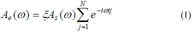
Ordaz et al., (1995) assumed two facts: the record of a single, small event represents Green's function for all points of the large earthquake's rupture area, and both earthquakes' source spectra obey the ω₂ scaling law. This method is aimed at devising an a_s(t) summation scheme for synthesising target event ground motion conforming to the ω₂ scaling law in the entire frequency band of interest. Ordaz et al. (1995) considered that target event source is divided into N cells, the jth of which generates, starting at time t_j, signal ξa_s(t), whose Fourier spectrum is ξA_s(w). The resulting signal spectrum, A_e(w), is:

If t_j's are random, independent and equally distributed with probability density function p(t), the expected value of |A_e(w)|², E[|A_e(w)|²], is given by:

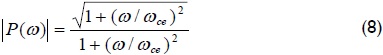
where P(w) is the Fourier transform of p(t). The expected Fourier spectral ratio between the resulting and the original signals, R(w), can be estimated with:

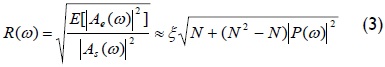
By definition, P(0)=1, hence R(0)=ξN. On the other hand, if |P(ω)| must vanish as ω→∞, then R(∞)=ξN^1/2. The assumption that the sources follow an ω² model implies that the spectral ratio of the target to the small event, H(ω), must be:

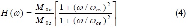
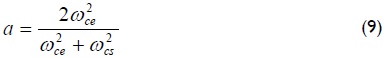
To match the lower and upper ends of spectral ratio H(ω) with those given by R(ω), parameters N and ξ in (3) should be given by:

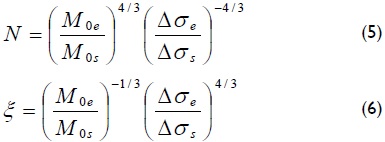
where Δσ is the stress parameter, related to ω_c by

where β is the S-wave in km/sec, M₀ is in dyne-cm and Δσ is in bar. With the values of N and ξ given in (5) and (6), the summation scheme yields correct scaling at very low and very high frequencies. At intermediate frequencies, however, R(ω) depends on P(ω) and hence on the choice of delay time probability distribution, p(t). If theoretical scaling must hold at all frequencies, then H(ω) must equal R(ω) for all frequencies. It then follows from (3) and (4) that:

with

An additional constraint is that P(ω) be real. In this case, the desired probability density function p(t) is given by:

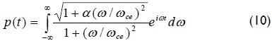
It should be noted that p(t) extends to infinity in both its tails, so rupture times simulated with this procedure could be negative. Moreover, there is nonzero probability of the total simulated rupture time being larger than rupture duration T_d = 2π/ω_ce. For a given simulation, however, the relative number of sub-events occurring outside the expected rupture window Td is very small. On the other hand, if p(t) were truncated to exclude all rupture times outside a certain window, then a box car function will be involved in the time domain and hence a sinusoidal function in the frequency domain. Consequently, holes would appear at some frequencies in the target event spectrum (Ordaz et al., 1995).

Experimental program

Reliable results regarding structures' seismic behaviour can be obtained by carrying out shake table tests which can statistically reproduce the characteristics of real earthquake motion in the time and frequency domains (Dowling, 2006).

Shake table tests of six specimens were aimed at better understanding the seismic performance of reinforced concrete walls for low-rise housing. Characteristic earthquake records were simulated using the empirical Green's function to define seismic demand during dynamic tests.

The three-dimensional prototype consisted of a two-story house built with reinforced concrete walls; this type of housing construction frequently involves using 100-mm thick solid slabs or slabs made of precast elements. Wall thickness and clear height are usually 100 mm and 2,400 mm, respectively, and house floor plan area varies between 35 and 65 m2. Foundations are strip footings made of RC 400-mm square beams supporting a 100-mm thick floor slab. The fundamental period of vibration of the prototype house was estimated to be equal to 0.12 s (8.3 Hz). Details of the experimental program may be found elsewhere (Carrillo and Alcocer, 2013, 2012).

Definition of earthquake records for dynamic tests

Earthquake ground motion is a stochastic phenomenon whose characteristics depend on source mechanism and local soil conditions. However, as a deterministic, dynamic phenomenon, an earthquake will never occur again in the same form. Hence, structures do not need to be tested by subjecting them to simulated ground motion, which is exactly the same as an actual earthquake record (Tomazevic and Velochovsky, 1995). However, earthquake motion records are the main source for testing structures under dynamic loading, like an earthquake. Therefore, one or various characteristic earthquake records may be chosen for scaling them and defining synthesised larger or lower severity earthquake motions. Most experimental studies consider variation of the motion severity by increasing the record at different peak ground acceleration values. However, earthquake motion severity is not only a function of the instrumental intensity but also of the frequency content, duration and the amount of energy imposed on the structure.

Three limit states were defined for assessing wall performance at different damage levels: onset of diagonal cracking, strength and near collapse. In this study, the Diagonal cracking limit is reached when the initial inclined web cracking was observed. The strength limit state is reached when the peak shear strength was attained. The near collapse limit is associated with one of the following scenarios: when a 20% drop in peak strength was observed or when web shear reinforcement became fractured.

The time-histories of 76 seismic events occurring in Mexico between 1960 and 1999, magnitude M ≥ 5 and peak ground acceleration PGA ≥ 0.3 g, were analysed to define the earthquake records to be reproduced on the shake table. Only seismic events recorded by stations on rock or on firm soil were evaluated for considering the prototype house's dynamic properties (short period structures, 0.12 s) and excluding the records' site effects. Elastic response spectra in terms of acceleration, velocity and displacement were calculated to evaluate the impact of the 76 earthquakes on prototype house performance.

Earthquake record for cracking limit state

A record concerning an earthquake occurred in the subduction area on Mexico's Pacific coast was found to induce the highest elastic displacement on the prototype house. The earthquake was recorded in the epicentral region near Acapulco, at the Caleta de Campos station, Mexico, on the 11^th of January, 1997. This record was used for seismic demand representing the diagonal cracking limit state. Santoyo et al., (2005) estimated a nearly-vertical faulting at a depth of 35 km, moment magnitude M_W of 7.1 moment magnitude, stress drop Δσ of 40 bar (» 40 kgf/cm2) and mean rupture velocity of 2.8 km/sec, from the inversion of teleseismic recordings of this event. The record's S90E horizontal component (PGA = 0.38 g) was used for shake table testing in this study.

Analysing the 76 earthquakes led to concluding that seismic events having a magnitude larger than that of events recorded between 1960 and 1999 in Mexico should be simulated to attain damage levels related to the prototype house's strength and near collapse limit states.

Events for strength and near collapse limit states

Large-magnitude seismic events, i.e. having larger instrumental intensity and duration, were simulated to study the performance of the specimens at different earthquake load levels. The M_W 7.1 record was considered an empirical Green's function for numerically simulating two earthquakes having M_W 7.7 and 8.3 related to strength and near collapse limit states, respectively. Earthquakes' stress drop Ds and seismic moment M₀ should be estimated to use the method of the empirical Green's function.

The M_W 7.1 seismic event's stress drop was also used for simulated seismic events (M_W 7.7 and 8.3). Seismic moment M₀ is a very important earthquake parameter measuring overall deformation at the source. M₀ is one of the most accurately determined seismic source parameters. Kanamori (1977) proposed using (11) for estimating the moment magnitude M_W from seismic moment M₀ (dyne-cm):

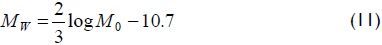
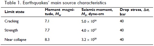
Seismic moment was calculated in this study by using Kanamori's equation. Table 1 shows recorded and simulated earthquakes' main source parameters.

Results of recorded and simulated events

Acceleration, velocity and displacement time histories for recorded and simulated earthquakes related to prototype house are shown in Figs. 1, 2 and 3, respectively.

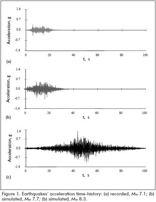
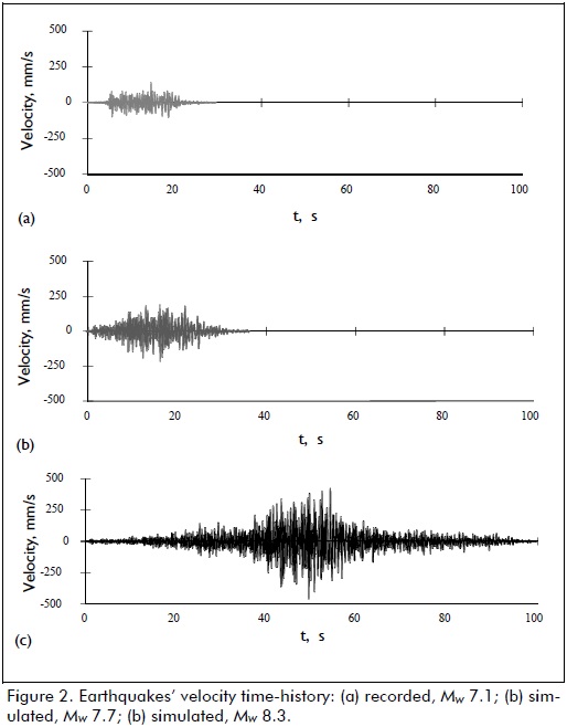
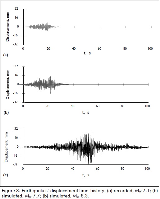
All signals were processed in time and frequency domains. A normal baseline correction was applied to the signals. Signals were also bandpass-filtered between 1 and 50 Hz using a four pole Butterworth filter. Maximum frequency was selected based on the characteristics of the instrument used for recording the M_W 7.1 event. Minimum frequency was selected for preserving the prototype structure's range of frequencies.

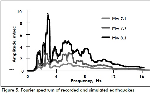
Acceleration, velocity and displacement response spectra for 5% damping, and Fourier spectra of acceleration time histories are also shown in Figs. 4 and 5, respectively. Peak ground acceleration (PGA), peak ground displacement (PGD), total duration and duration of the strong phase of recorded and simulated earthquakes are presented in Table 2.

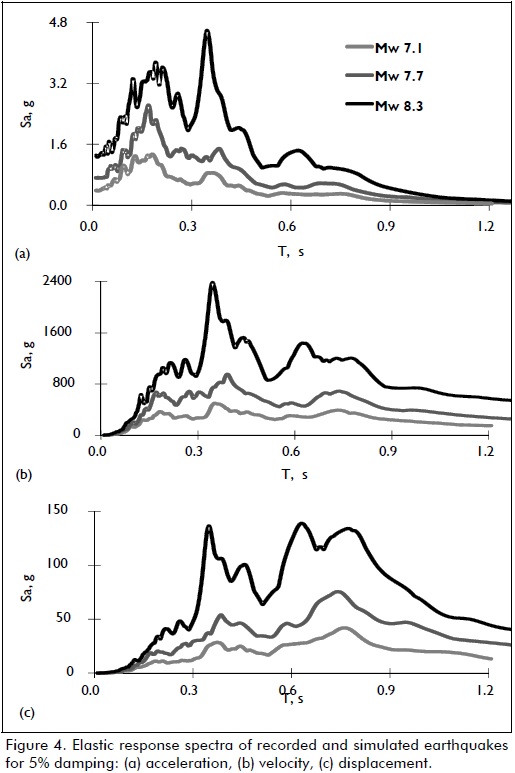
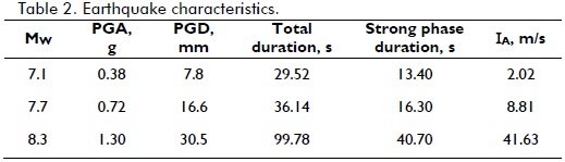
Arias' (1970) intensity factor IA was calculated for verifying earthquakes' increasing instrumental intensity. IA values are also included in Table 2. This factor has been shown to be a good estimator of damage because it reveals earthquake-loading history in terms of intensity and duration. Arias intensity is a measure of the potential earthquake destructiveness associated with acceleration time history. Factor IA is calculated by:

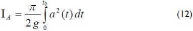
where a is ground acceleration in a given direction, t₀ is the total earthquake duration of the earthquake and g is the acceleration due to gravity. As shown in Table 2, the increasing earthquake instrumental intensity was attained using the proposed method.

Discussion of results

Green's function as a tool for simulating events

Estimation of ground motions for a future earthquake is a fundamental step in anticipating possible damages and trying to mitigate devastating concomitant devastating effects. However, the subsoil in many regions is not sufficiently known for simulating wave propagation at a relevant frequency band for earthquake-engineering purposes (between 0.1 and 40 Hz). An attractive approach for overcoming this problem is to sum the recordings of small earthquakes delayed between each other to reproduce the rupture propagation effect. Each small-earthquake recording represents all the propagation effects between the source and the receiver and is then regarded as an empirical Green's function. This method has the advantage of incorporating both wave-propagation and site effects (Hartzell, 1978; Kohrs-Sansorny et al., 2005).

The event seismic moments and stress parameters of the empirical Green's function and the target event must be specified for simulating motion with an empirical Green's function. It is thus reasonable to assume that empirical Green's function moment and stress parameters are known. Since target event magnitude (hence the seismic moment) is necessarily specified, only its stress parameter is free. One alternative in choosing the target event stress parameter is to take its value as equal to that of the empirical Green's function. This may give a conservative estimate, since evidence (e.g. Ordaz and Singh, 1992) seems to suggest that large earthquakes' stress parameters are usually smaller than those for small earthquakes (Ordaz et al., 1995).

Validation of similar testing conditions

Recorded and simulated earthquakes' acceleration response spectra are shown in Figure 6(a). The range of periods related to highest spectral intensity is highlighted by a box-shaped marker in the Figure. Although two ranges of dominant periods were observed for the seismic event associated with near collapse limit state, only the range closest to the specimens' periods of vibration is highlighted in Figure 6(a).

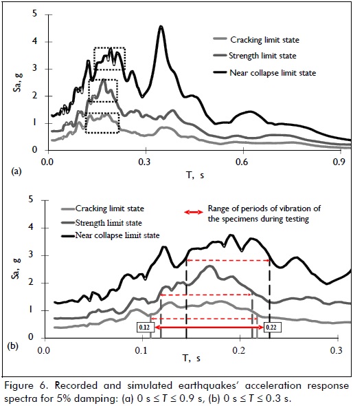
Acceleration response spectra between T = 0 s and T = 0.3 s are shown in Figure 6(b). Estimation of the range of specimens' periods of vibration of vibration during testing is depicted in the Figure. As indicated earlier, the fundamental period of vibration of the prototype house is 0.12 s (8.3 Hz). Such period is close to the lower value of the range of dominant periods of the seismic event associated with cracking limit state (0.11 s). If the specimens' maximum stiffness degradation during all testing stages is 70%, then the specimen's final period of vibration is 0.22 s. This period is close to the upper value of the range of dominant periods of the seismic event associated with the near collapse limit (0.23 s).

The range of periods having higher spectral intensity in recorded and simulated earthquake signals in this study was comparable to the range of specimens' periods of vibration during all testing stages. The three defined objectives for shake table testing were thus fulfilled from initial to final testing stages for each specimens, i.e. dynamic similitude by establishing the specimen' periods of vibration comparable to the earthquake spectrum dominant periods, assessing specimens damage under conditions close to dynamic resonance, and comparing specimens' response under gradual increment of the seismic intensity by unchanging record duration.

Conclusions

The following conclusions were drawn from this study:

The small event regarding empirical Green's function should be infinitely small for starting from a "point fault" and thus really represent Green's function. However, the small event must be strong enough to generate amplitudes at low frequencies well above both ground noise level and instrumental resolution. In practice, the event is only small regarding the target event.

Most experimental programs assessing structures' dynamic performance consider variation of the motion severity by increasing the record to different peak ground acceleration values, until the near collapse limit state is attained. However, earthquake motion severity is not only a function of the instrumental intensity but also of the frequencies content, duration and the amount of energy imposed on the structure.

Three or more signal events characterising the seismic area and fulfilling particular requirements should be selected for satisfying dynamic test conditions. An earthquake record should be considered an empirical Green's function for simulating large-magnitude events for selecting particular signal events, i.e. having larger instrumental intensity and duration. The proposed method has not been used for shake table testing of specimens according to a review of the pertinent literature.

References

Arias, A., A measure of earthquake intensity., In: Seismic design for nuclear power plants., MIT Press, 1970, pp. 438-483.         [ Links ]

Carrillo, J., Alcocer, S., Simplified equation for estimating periods of vibration of concrete wall housing., Engineering Structures, Vol. 52, 2013, pp. 446-454.         [ Links ]

Carrillo, J., Alcocer, S., Seismic performance of concrete walls for housing subjected to shaking table excitations., Engineering Structures, Vol. 41, 2012, pp. 98-107.         [ Links ]

Dowling, D., Seismic strengthening of adobe-mudbrick houses., PhD Thesis, University of Technology, Sydney, Australia, 2006.         [ Links ]

Hartzell, S., Earthquake aftershocks as Green's functions., Geophysical Research Letters, Vol. 5, No. 4, 1978, pp. 1-4.         [ Links ]

Kanamori, I., The energy release in great earthquakes., Geophysical Research, Vol. 82, No. 20, 1977, pp. 2981-2988.         [ Links ]

Kohrs-Sansorny, C., Courboulex, F., Bour, M., Deschamps, A., A two-stage method for ground-motion simulation using stochastic summation of small earthquakes., Bulletin of the Seismological Society of America, Vol. 95, No. 4, 2005, pp. 1387-1400.         [ Links ]

Koller, M., Lachet, C., Fourmaintraux, D., Seismic hazard assessment with the aid of emprirical Green's functions., Proc. 11th World Conference on Earthquake Engineering, Acapulco, Mexico, paper 724, 1996.         [ Links ]

Ordaz, M., Singh, S., Source spectra and spectral attenuation of seismic waves from Mexican earthquakes, and evidence of amplification in the hill zone of Mexico City., Bulletin of the Seismological Society of America, Vol. 82, 1992, pp. 24-43.         [ Links ]

Ordaz, M., Arboleda, J., Singh, S., A scheme of random summation of an empirical Green's function to estimate ground motions from future earthquakes., Bulletin of the Seismological Society of America, Vol. 85, No. 6, 1995, pp. 1635-1647.         [ Links ]

Santoyo, M., Singh, S., Mikumo, T., Source process and stress change associated with the 11 January, 1997 (Mw = 7.1) Michoacan, Mexico, inslab earthquake., Geofísica Internacional, Vol. 44, No. 4, 2005, pp. 317-330.         [ Links ]

Tomazevic, M., Velochovsky, R., Some aspects of experimental testing of seismic behavior of masonry walls and models of masonry buildings., Earthquake Engineering and Structural Dynamics, Vol. 21, No. 11, 1992, pp. 945-963.         [ Links ]